3. Problem formulation

3.1 The mechanism and its specification

The linkage follows Honda’s EXlink topology with two changes, each of which frees a dimension to optimise: a crank is inserted between the half-speed shaft and the swing rod, and another between the crankshaft and the trigonal link.

The shaft arrangement is Honda’s. The crankshaft carries the crank that drives the trigonal link and turns twice per cycle, exactly as on a conventional four-stroke; the half-speed shaft carries the swing-rod crank and turns once. Power is taken from the crankshaft, so an engine speed quoted here means what it means for any other four-stroke, and the comparison of §5.4 is at equal speed and equal firing rate with no correction of any kind.

The engine data are those of a Shell Eco-marathon prototype-class single cylinder:

quantity	symbol	value
bore	\(\Phi\)	32 mm
expansion stroke	\(\mathrm{STE}\)	74 mm (required)
compression ratio	\(\varepsilon\)	16 (required)
clearance volume	\(V_0\)	3 cm³
plenum pressure	\(P_0\)	1.2 bar
combustion pressure ratio	\(k = P_3/P_2\)	1.7
polytropic exponent	\(\gamma\)	1.22
piston length, pin to crown	\(p\)	16 mm
maximum piston-rod tilt	\(\mathrm{mra}\)	10°
gear ratio, half-speed shaft to crankshaft	\(r_1/r_2\)	2

\(\varepsilon = 16\) is high enough to knock on pump fuel; the target assumes variable valve phasing and a suitable fuel, and is treated here purely as a geometric requirement. With \(\Phi = 32\) mm and \(V_0 = 3\) cm³ it pins the compression stroke at \(\mathrm{STC} = 15V_0/A_p \approx 55.95\) mm against the required \(\mathrm{STE} = 74\) mm — the asymmetry the linkage exists to produce.

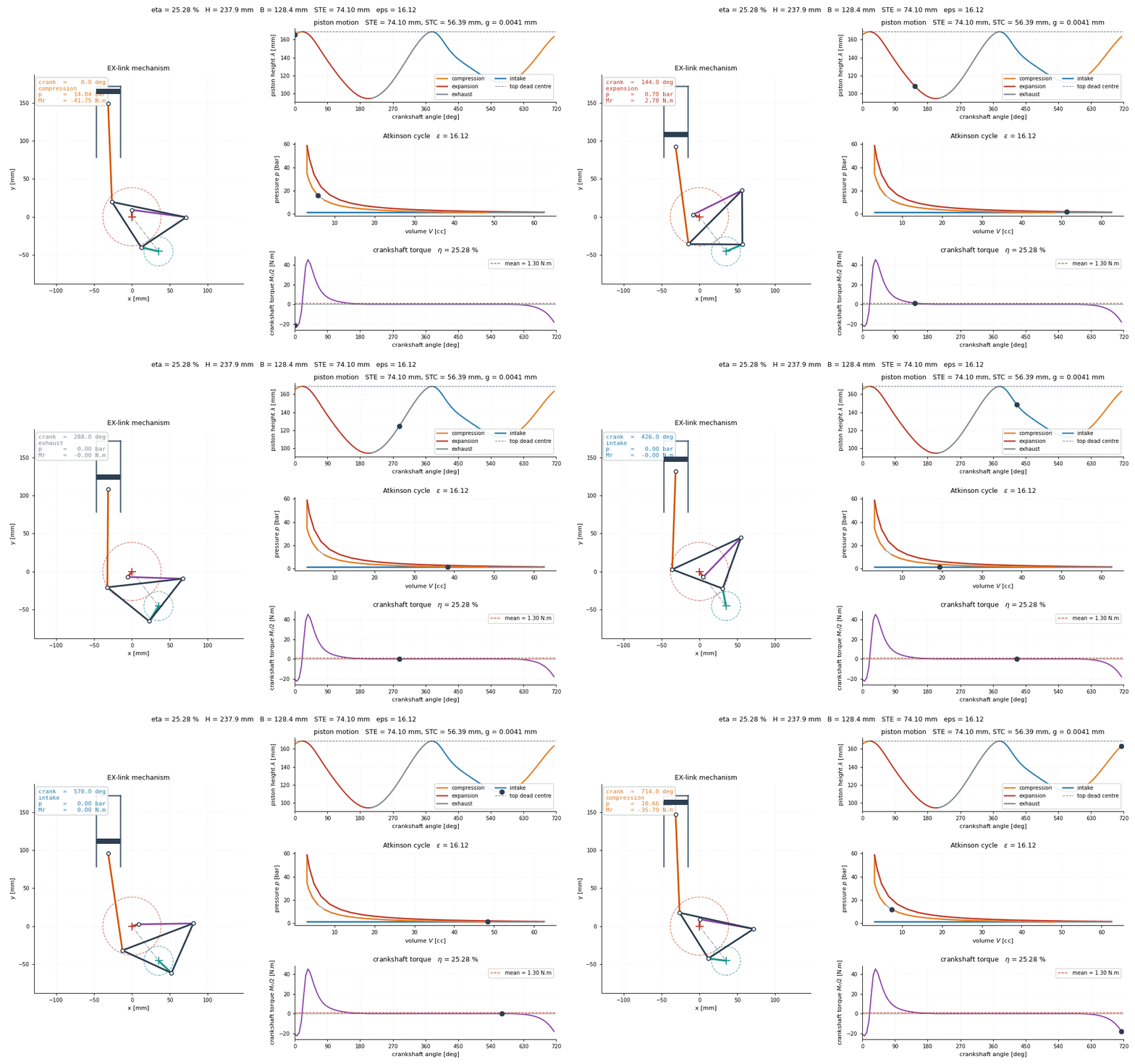
The design of §5.5 through one cycle: 360° of the half-speed shaft, 720° of the crankshaft. Left, the linkage; right, piston height, the \(p\)–\(V\) cycle and crankshaft torque, with a marker tracking the crankshaft angle on each. Every abscissa runs over the 720° the cycle spans, so these read against a conventional four-stroke’s without conversion.

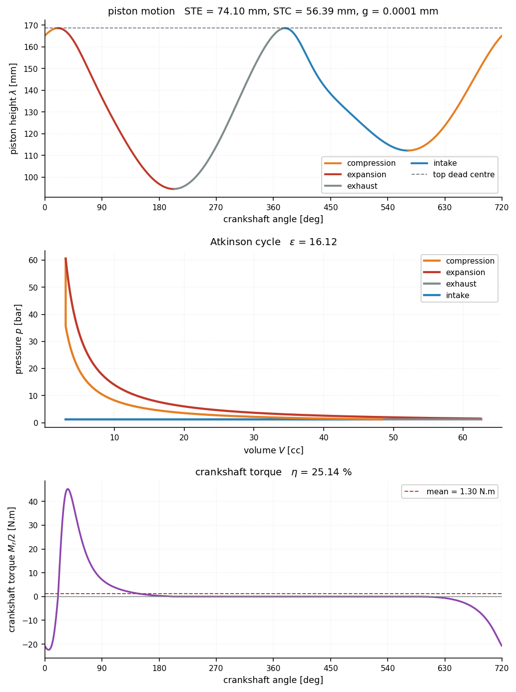
The piston reaches the same top dead centre twice per cycle — 360° of crankshaft apart — but two different bottom dead centres. Torque is strongly positive through expansion, negative through compression, and flat through intake and exhaust, where the cylinder is at plenum pressure and the piston carries no gas load.

3.2 Design variables and objective

Eleven continuous dimensions describe the linkage:

\[X = (a,\; c,\; I,\; x_b,\; y_b,\; x_1,\; e,\; q_1,\; q_2,\; \theta_f,\; \theta_r)^{\mathsf T}. \tag{3.1}\]

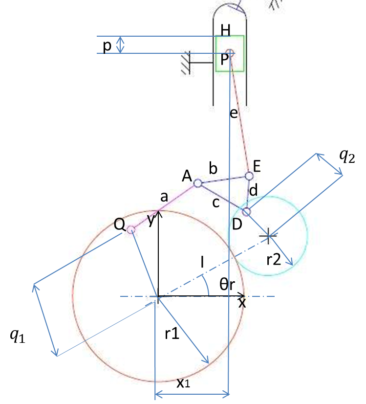
The parametrisation. \(R_1\) carries the crank \(q_1\) ending at \(Q\) and the large gear of pitch radius \(r_1 = 2I/3\); \(R_2\) carries \(q_2\) ending at \(D\) and the small gear \(r_2 = I/3\), and sits at distance \(I\) in the direction \(\theta_r\) measured from \(+x\). The swing rod \(a\) runs \(Q \to A\), the trigonal link is the triangle \(A\text{–}D\text{–}E\) with sides \(b\), \(c\), \(d\), the piston rod \(e\) runs \(E \to P\), and the crown \(H\) sits \(p = 16\) mm above \(P\) on the cylinder axis, offset \(x_1\) from the \(R_1\) axis. Ten of the eleven appear here; the eleventh, the dephasing \(\theta_f\), cannot be drawn on a single pose, being the constant in \(\theta_2 = -2\theta_1 + \theta_f\) — and \(\theta_1\) and \(\theta_2\) are measured from \(+y\) rather than from \(+x\) (Appendix A §A.1).

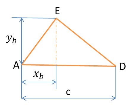
Two of the eleven replace \(b\) and \(d\). Describing the triangle by its three sides would force the design space to respect the triangle inequality and would leave the sign of the apex undetermined; placing \(E\) at \((x_b, y_b)\) in the frame with origin \(A\) and first axis along \(AD\) lets both range freely over \(\mathbb R\) and makes the design space a plain box.

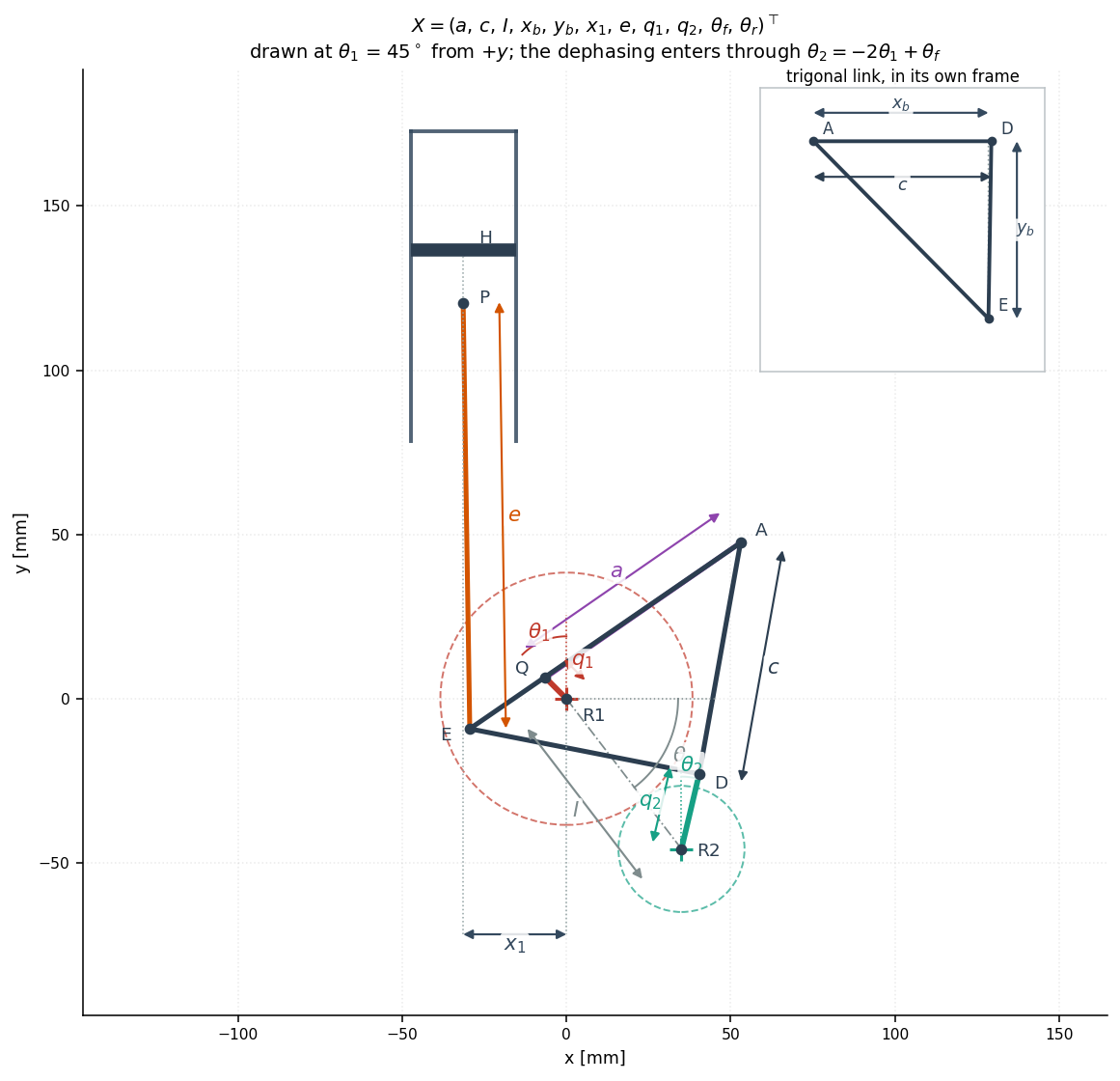
The same eleven on the design of §5.5, frozen at \(\theta_1 = 45^\circ\) — proportions to scale rather than schematic, which is why \(q_1\) is so much shorter than the sketch above suggests.

\(a\)	swing rod \(QA\)
\(c\)	side \(AD\) of the trigonal link
\(x_b\), \(y_b\)	position of \(E\) in the frame carried by \(AD\)
\(e\)	piston rod \(EP\)
\(q_1\), \(q_2\)	cranks on the half-speed shaft and on the crankshaft
\(I\)	distance between the two shafts
\(x_1\)	lateral offset of the cylinder axis
\(\theta_f\), \(\theta_r\)	crank dephasing, and shaft-axis orientation

§2.2 rejects the conventional objective. The objective used here is the quantity the application scores,

\[\max_X \; R(X) \quad [\mathrm{km/L}], \tag{3.2}\]

which requires the chain

\begin{equation} X \longrightarrow \lambda(\theta_1) \longrightarrow p(V) \longrightarrow \text{loads} \longleftrightarrow \text{sections} \longrightarrow \begin{cases} W_{\mathrm{brake}} \\ m_{\mathrm{engine}} \end{cases} \longrightarrow R. \tag{3.3} \end{equation}

Range prices the competing quantities at rates the physics fixes rather than the designer: a point of brake efficiency is worth a fixed distance through the fuel burnt per unit work; a millimetre of envelope is worth a fixed mass of crankcase, and a kilogram a fixed distance through rolling resistance; a newton-millimetre of torque ripple is worth a fixed mass of flywheel.

3.3 Evaluating the objective

The objective is not a formula but a chain. Each link is a first-order model, and each is checked in §4.9 against a result computed independently of it.

Motion and cycle. The loop-closure equations are inverted analytically rather than solved with Newton–Raphson, which matters twice: the evaluation is fast, and the two arccosine arguments it exposes become the well-posedness conditions

\[\delta_{c1} \le 1, \qquad \delta_{c2} \le 1, \qquad W = \max(\delta_{c1}, \delta_{c2}), \tag{3.4}\]

that keep the linkage assemblable. \(W \to 1\) is the transmission-angle singularity §5.1 turns on. Before pressure is assigned, \(\lambda(\theta_1)\) must be shown to have exactly four monotone phases — two maxima and two distinct minima — which is what makes the motion Atkinson rather than a stair-stepped artefact. The cycle is then adiabatic compression and expansion about a constant-volume heat release,

\[Q = \frac{V_0(P_3 - P_2)}{\gamma - 1}, \tag{3.5}\]

with \(Q\) fixing the fuel consumed. Deriving the fuel from the heat release keeps the range model consistent with the thermodynamics rather than bolting a second combustion model alongside it.

Mechanical losses. §2.2 notes that \(\eta\) loses nothing. The real losses come from quantities the equilibrium solve already produces — joint reactions \(R_j\) turning through relative angles \(\Delta\theta_j\), and the liner reaction \(D\) the side-load constraint already bounds:

\[W_{\mathrm{bearings}} = \sum_j \mu_j r_j \oint |R_j| \left|\frac{\mathrm{d}(\Delta\theta_j)}{\mathrm{d}\theta_1}\right| \mathrm{d}\theta_1, \tag{3.6}\]

\[W_{\mathrm{piston}} = \mu_p \oint \bigl(|D| + F_{\mathrm{ring}}\bigr) \left|\frac{\mathrm{d}\lambda}{\mathrm{d}\theta_1}\right| \mathrm{d}\theta_1. \tag{3.7}\]

This is what makes the constraint set mean something. Without it the side-load and bearing-load bounds are assertions about wear that never enter any objective; with it, a design that leans on the liner burns its fuel on the liner.

Engine mass. The sized members weigh 0.15 kg, and no engine weighs 0.15 kg; optimising that number optimises a tail. The budget carries eight items, of which two change the shape of the problem rather than its scale. The crankcase converts the envelope into kilograms — a box encloses the mechanism and its walls scale with \(H \times B\), so the two envelope objectives of §2.2 become mass at a rate the physics fixes. The flywheel converts torque ripple into kilograms,

\[J = \frac{\Delta E}{\delta\,\omega^2}, \qquad \Delta E = \max_\theta E(\theta) - \min_\theta E(\theta), \qquad E(\theta) = \int_0^\theta (M_r - \bar M_r)\,\mathrm{d}\theta_1, \tag{3.8}\]

so a linkage whose torque curve is flatter is lighter — a driver no geometric constraint expresses, pushing against a long lever arm. The turning-moment diagram here must be the gas torque: the inertia part is energy traded with the mechanism’s own masses, already accounted for by the inherent rotating inertia, and including it overstates the flywheel fivefold at low speed.

Sizing, and the coupling it creates. Nothing in \(X \to \lambda \to p \to \text{loads}\) determines a cross-section, and without sections there is no mass, without mass no inertia, and (3.2) cannot be evaluated at all. Sizing the members against yield, fatigue and buckling closes that gap, but the sizing needs the loads and the loads need the masses, so with \(d\) the section diameters and \(N, M\) the internal loads,

\[d = \mathcal{S}\bigl(N(d),\, M(d)\bigr) \tag{3.9}\]

is a fixed point rather than a sequence. It has one, and plain iteration reaches it (§A.9). The cubic dependence of the fixed point on acceleration is why engine speed dominates the answer, and why the problem is multidisciplinary in the strict sense — §4.3 must choose an architecture for it.

From engine to distance. These cars are driven burn and coast: run hard from \(v_{lo}\) to \(v_{hi}\), declutch, coast back. With \(Mv\,\mathrm{d}v/\mathrm{d}x = F\),

\[d = \int_{v_{lo}}^{v_{hi}} \frac{Mv\,\mathrm{d}v}{F(v)}, \qquad t = \int_{v_{lo}}^{v_{hi}} \frac{M\,\mathrm{d}v}{F(v)}, \tag{3.10}\]

with \(F = P_w/v - F_{\mathrm{res}}\) under power and \(F = F_{\mathrm{res}}\) coasting. Over one closed cycle the car starts and ends at the same speed, so the kinetic energy nets to zero and the propulsive work equals the resistance work over the whole distance: hard acceleration costs nothing in road load. What the strategy buys is that the engine runs at high load; what it costs is aerodynamic. The minimum-average-speed rule is active at every optimum where the engine has power to spare, which collapses the two-dimensional strategy search to one dimension — and matters beyond speed, since a grid search would make the objective a step function of the design variables and the optimizer downstream would be differentiating quantisation noise.

3.4 Settings, and the baseline

The disciplines are evaluated at the following settings unless stated otherwise. Each is a resolution or modelling choice rather than a design variable.

setting	value	why
samples per cycle	360 (coupled), 720 (reporting)	the top-dead-centre gap needs 360 or more to be measured correctly
stations along each member	9	internal loads are cubic in the station coordinate
material	42CrMo4 Q&T	\(S_y = 700\) MPa, \(S_u = 900\) MPa
safety factors	1.5 static, 2.0 fatigue, 2.5 buckling	first-iteration structural practice
journal friction coefficient	0.008	hydrodynamic, warm
speed fluctuation for the flywheel	0.10	road vehicle with a clutch
machining tolerance	ISO 286 IT8	machined linkage member
vehicle	35 kg glider, 50 kg driver	Prototype class; the driver minimum is a competition rule
engine speed	2000 rev/min at the crankshaft	1000 cycles per minute; §5.1 sweeps it

Engine speeds are quoted at the crankshaft throughout, which turns twice per cycle on both mechanisms. The speed_rpm the analysis functions take is the half-speed shaft’s, because that is the shaft the kinematics are parametrised on. The engine is 12.5 % of the 97 kg rolling mass, so a kilogram of engine is worth 13.6 km/L — the exchange rate (3.2) relies on.

A design vector from an earlier unpublished study of the same mechanism is carried as a starting point, not as a result. Re-analysed as printed it violates five constraints, most tellingly a top-dead-centre gap of 8.5 mm against a 0.01 mm bound. Rounding does not explain it: perturbing each variable by its four-significant-figure half-width moves the stroke by less than 0.2 mm. The explanation is conditioning — the vector sits at \(W = 0.982\), where the piston motion is violently sensitive to the link lengths, so the design is not reproducible to four digits across two independent implementations. It is the first appearance of the theme §5.1 develops.

3.5 The specification cannot be met as written

Two of the seven requirements in §3.1 are equalities, and that is a property of this specification rather than of mechanism synthesis in general. Most dimensional-synthesis problems bound their requirements; this one fixes the expansion stroke at 74 mm and the compression ratio at 16 exactly, because both were written as targets before any part existed. The consequence is geometric: the two equalities cut the eleven-dimensional design box down to a nine-dimensional manifold, so the feasible set has Lebesgue measure zero and a point drawn at random lies off it with probability one.

The defect is in the statement rather than in the mechanism. A requirement given as an equality cannot be met by a manufactured part: no dimension is produced exactly, so the stroke of a built engine is a random variable and \(\mathrm{STE} = 74\) is a requirement no engine has ever satisfied. Restoring what the equality was shorthand for gives

\[|\mathrm{STE} - 74| \le \delta_{\mathrm{STE}} = 0.05\ \mathrm{mm}, \qquad |\varepsilon - 16| \le \delta_\varepsilon = 0.05, \tag{3.11}\]

with the half-widths taken from what a machined linkage member holds. The feasible set becomes full-dimensional and the problem well posed, and it is (3.11) rather than the equalities that the rest of this document solves.

Two things follow, and the study returns to each. The relaxation is a promise about tolerance, and a promise that can be checked: §4.5 compares the bands with the scatter of the parts they are supposed to cover, and §5.2 prices what widening them costs and buys. And a feasible set of measure zero excludes an entire class of optimizer before any is tried, which §4.1 measures.