4. Method

Every element of the method below is forced by a property of the formulation of §3 rather than chosen for convenience. Each subsection states the property, what it excludes, and what it leaves.

4.1 The feasible set is thin, and that selects the optimizer

§3.5 relaxed the two equality requirements into bands (3.11), and the feasible set is full-dimensional as a result. It is not, however, wide: the bands are 0.05 mm and 0.05 on quantities the design variables move by millimetres, so what was a measure-zero manifold is now a sliver around one. That is enough to change which optimizers can be used and not enough to let a sampling method work, and both halves are measurable rather than asserted.

method	outcome
COBYLA from the reference design	120 evaluations, 313 s, returns its input unchanged
4000 uniform samples over the global box	0 feasible
4000 uniform samples within 50 % of a feasible design	0 feasible
4000 uniform samples within 10 % of a feasible design	0 feasible

Only a method that moves along the manifold is admissible, which selects sequential quadratic programming with exact gradients — and makes §4.2 necessary rather than merely desirable. The same thinness returns twice more: it is why the restarts of §4.6 have to be constructed on the manifold rather than drawn, and it is what defeats the line search when a reliability constraint is attached to a search whose other constraints are not imposed (§4.7).

4.2 Finite differences are wrong, not merely inaccurate

Several constraints are extrema over the crank revolution,

\[\gamma(X) = \max_{\theta_1} \frac{|D(X,\theta_1)|}{\max_{\theta_1}|P(\theta_1)|}, \tag{4.1}\]

and the sample attaining the maximum changes as \(X\) moves. A difference quotient taken across that switch does not approximate a derivative: it is measured at 25 % error on \(\gamma\) at a \(10^{-4}\) mm step, and it does not improve as the step is reduced.

Because the chain of §3.3 is closed form, derivatives propagate forward alongside each intermediate, and for an extremum attained at \(\theta^\ast\) the envelope theorem gives

\[\frac{\mathrm{d}}{\mathrm{d}X}\Bigl[\max_\theta f(X,\theta)\Bigr] = \frac{\partial f}{\partial X}\Bigr|_{\theta^\ast}, \tag{4.2}\]

the term through \(\mathrm{d}\theta^\ast/\mathrm{d}X\) vanishing because \(\partial f/\partial\theta = 0\) at the maximiser. The switching problem disappears rather than being mitigated.

The same idea applies twice more inside the fixed point (3.9). The \(18\times18\) equilibrium solve differentiates as

\[\frac{\partial x}{\partial p} = A^{-1}\Bigl(\frac{\partial b}{\partial p} - \frac{\partial A}{\partial p}\,x\Bigr), \tag{4.3}\]

reusing the factorisation already computed; and the sizing bisection is never differentiated at all, because the diameter is defined implicitly by \(U(d, N, M) = 1\), so

\[\frac{\partial d}{\partial q} = -\frac{\partial U/\partial q}{\partial U/\partial d}. \tag{4.4}\]

SLSQP thus becomes applicable to a problem on which derivative-free search returns its input. Derivations are in Appendix A §A.10.

4.3 The coupling is a field, not a handful of scalars

The fixed point (3.9) leaves a multidisciplinary analysis to be placed, and the MDF/IDF trade is decided by the dimension of the coupling:

\[\dim(\text{coupling}) = \underbrace{2 \times 7 \times 360 \times 9}_{\text{load histories}} + \underbrace{7}_{\text{diameters}} + \underbrace{1}_{\text{piston mass}} = 45\,368 \tag{4.5}\]

against eleven design variables. The couplings are not scalars but the internal load history of every member at every crank angle at every station. IDF would carry 45 367 extra design variables and as many consistency constraints in order to optimise eleven degrees of freedom; it is not slower but unavailable, so the architecture is MDF.

How strongly coupled the problem is can be measured rather than asserted: Gauss–Seidel converges linearly at a rate that is the coupling strength, \(\rho = \lim_k \lVert r_{k+1}\rVert / \lVert r_k\rVert\). At rest \(\rho = 0\) exactly — with no inertia there is no path from mass to load, and the quasi-static problem is recovered — rising to 0.68 at 3000 rev/min (Appendix C).

4.4 The gear choice is discrete and pins a design variable

A gear has an integer tooth count cut with a standard-module hob. For the 2:1 pair, \(r = mz/2\) and \(z_1 = 2z_2\), so

\[I = \tfrac32 m z_2, \qquad m \in \text{ISO 54}, \quad z_2 \in \mathbb Z,\ z_2 \ge 17. \tag{4.6}\]

\(I\) lives on a lattice rather than an interval, and \(I\) is one of the variables the equalities are satisfied with, so choosing the gears throws the design off both: a 0.18 mm snap to the nearest lattice point moves the top-dead-centre gap from 0.003 mm to 0.058 mm.

The problem is stated as the mixed-integer nonlinear program it is and decomposed. Outer approximation is chosen over generalised Benders because of what each master requires: a Benders cut needs the optimal-value sensitivity \(\mathrm{d}\theta/\mathrm{d}I\), which requires multipliers this problem’s degenerate active set does not supply, whereas an outer-approximation cut needs only \(\nabla f\) and \(\nabla g\) at the visited point, which §4.2 already provides exactly. With \(y\) a one-hot selection over the lattice the master is

\begin{equation} \min_{x,y,\eta}\ \eta \quad\text{s.t.}\quad \begin{cases} \eta \ge f_k + \nabla f_k^{\mathsf T}(x - x_k), \\ 0 \ge g_k + \nabla g_k^{\mathsf T}(x - x_k), \\ I = \sum_j I_j y_j, \quad \sum_j y_j = 1. \end{cases} \tag{4.7} \end{equation}

Infeasible sub-problems need no special machinery: their constraint linearisations are added without an objective cut, which excludes that lattice point on evidence.

4.5 The relaxed bands are comparable with the scatter

The bands (3.11) are a promise about tolerance, and the promise can be checked. With \(\Sigma\) the covariance of the dimensional errors and \(\nabla g\) from §4.2,

\[\sigma_g = \sqrt{\nabla g^{\mathsf T}\,\Sigma\,\nabla g}. \tag{4.8}\]

At IT8 machining tolerances the band half-width is \(\delta_{\mathrm{STE}} = 0.050\) mm against a scatter \(\sigma_{\mathrm{STE}} = 0.029\) mm, giving a best achievable capability index \(\delta/\sigma = 1.7\) and 0.68 at the reference design. The band is under two standard deviations wide, so a perfectly centred design misses it about 9 % of the time. The relaxation that made the problem solvable is the same quantity that makes it unreliable, and a deterministic optimizer satisfying \(|\mathrm{STE}-74| \le 0.05\) has no way to notice.

A fixed margin \(g + k\sigma_g \le 0\) per constraint is the wrong repair, because it is a reliability statement only under independence: here every constraint is a function of the same eleven dimensions, the measured correlations reach 0.94, and the two sides of a relaxed band are correlated at exactly \(-1\). What is constrained instead is a probability of failure that keeps the correlation,

\[P_f = 1 - \Phi_n(\beta;\rho) \le p_{\text{target}}, \qquad \beta_i = -\frac{g_i}{\sigma_i}, \qquad \rho_{ij} = \frac{\nabla g_i^{\mathsf T}\Sigma\nabla g_j} {\sigma_i \sigma_j}, \tag{4.9}\]

a first-order (FORM) index per constraint combined through the multivariate normal orthant. It costs one Jacobian evaluation, so it can sit inside the optimization; sampling is the reference against which it is checked, and §5.3 reports what that check found.

Which constraints the probability covers. The uncertainty model is \(\Sigma = \operatorname{diag}(\sigma^2)\) over the eleven dimensions, from ISO 286 grades plus an angular clocking term. It contains no material, load or friction scatter, and that fixes which constraints can honestly carry a probability: the seven that are functions of the eleven dimensions alone — the two bands and \(\mathrm{mra}\), \(W\), \(g\), \(d\), \(\gamma\) — for which \(\Sigma\) is the complete uncertainty and \(\beta = -g/\sigma\) means what it says. The remaining five are excluded for three different reasons. Slenderness is a category error rather than a gap: it fires when a link grows thicker than a third of its length, at which point sizing it as a beam has stopped being credible, and there is no probability that beam theory applies. Saturation is a genuine limitation, FORM linearising \(g\) at a ceiling where the linearisation carries no information. Bearing, “engine runs” and “gears fit” are load-dependent, and the missing ingredient is the uncertainty model rather than the derivative. A probability of failure computed from a model that omits the dominant source is worse than a deterministic margin, because it launders a partial variance into something that reads as a reliability statement and then enters the system union of (4.9). §5.3 widens \(\Sigma\) and reports what the wider model changes.

4.6 The problem is nonconvex

Everything above yields one local solution, and the global strategies all require feasible starting points, which §4.1 shows uniform sampling cannot produce. Restarts are therefore constructed on the manifold: perturb the incumbent, project the perturbation back onto the two equalities by a minimum-norm Newton step from the analytic Jacobians,

\begin{equation} \Delta X = -J^{+} r, \qquad J = \begin{bmatrix}\nabla\mathrm{STE}\\ \nabla\varepsilon\end{bmatrix}, \tag{4.10} \end{equation}

and let the optimizer restore the inequalities from there. This is a local-search diversification, not a global method; §5.5 reports what it settles and what it does not.

4.7 The problem solved

\begin{equation} \begin{aligned} \max_{X,\,y} \quad & R(X, y) && \text{range [km/L]} \\ \text{s.t.}\quad & g_i(X) \le 0, \quad i \in \{\mathrm{mra},\, W,\, g,\, d,\, \gamma\} && \text{geometric} \\ & |\mathrm{STE}(X) - 74| \le \delta_{\mathrm{STE}}, \quad |\varepsilon(X) - 16| \le \delta_\varepsilon && \text{relaxed equalities (3.11)} \\ & s(X, y) \le 0,\; \ell(X, y) \le 0,\; b(X, y) \le 0 && \text{saturation, slenderness, bearing} \\ & r(X, y) \ge 0, \quad h(X, y) \ge 0 && \text{engine runs, gears fit} \\ & I = \tfrac32 m z, \quad m \in \text{ISO 54},\ z \in \mathbb Z,\ z \ge 17 && \text{catalogue (4.6)} \\ & X \in [X_{lb}, X_{ub}] \subset \mathbb R^{11} \end{aligned} \tag{4.11} \end{equation}

Twelve constraints, with \(y\) the converged MDA state of §4.3. Two details the code makes visible and the notation does not: each two-sided band is attached as a pair of one-sided inequalities, so the scenario carries fourteen constraint functions for these twelve constraints; and \(I\) is an output of the catalogue relation rather than a free variable, leaving ten in the search. The envelope bounds \(H\) and \(B\) of §2.2 are not among the constraints at all — once the objective prices size through mass, a separate limit on it is redundant.

Imposed, or merely checked. Whether an optimizer is made to hold (4.11) is a separate question from stating it, and the study answers it both ways.

	coupled and vehicle rows	reliability	results
build_range_scenario()	bind only at the end	audited after	§5.1 – §5.4
maximise_range_from_target()	imposed at every step	audited after	§5.5
the same, with beta_target	imposed at every step	constrained	§5.5

The difference is not academic: the same SLSQP on the same problem reaches 4.9 % further under the second form and 1.7 % under the third, which also holds a reliability target the other two only measure. A constraint that binds only at the end lets the search spend its whole trajectory in a region it will later be told it cannot use.

Why the objective needs a fallback. \(R\) is not computable everywhere: a design whose kinematics closes can still fail to size, fail to run, or fail to produce a four-stroke motion, and at such a point the objective has no value for a line search to descend. A constant penalty leaves a flat region with no gradient. The objective is therefore a ladder, with a prescribed motion \(\lambda^\star\) holding its middle rung — range computable scores \(-R(X)\); analysable but with no range scores a floor plus \(\lVert\lambda(X)-\lambda^\star\rVert^2\); a motion that is not a four-stroke cycle scores a larger constant. Each rung is strictly worse than the one above, so the search is pushed back towards designs that run, and on the middle rung it still has something to follow. The target is a fallback rather than a constraint: it satisfies both equality requirements exactly, being a functional of \(\lambda\) alone, and it is abandoned the moment the range becomes computable.

Reliability, imposed. Under either of the first two forms the problem is deterministic and (4.9) is applied to the solution. The third form closes the loop by attaching FailureProbabilityDiscipline and a thirteenth constraint. Three things had to be true before that constrained problem could be solved, and each was found by a run that failed.

The other constraints must be imposed too. From the coupled reference design at \(\beta_{\text{sys}} = -0.422\), SLSQP under the first form returns its starting point unchanged — not only for a demanding target but for \(\beta \ge -0.2\), a step of 0.17 — reporting a positive directional derivative for the line search. The reliability gradient is not at fault; what defeats the line search is the thinness §4.1 measures. A step of 0.05 mm along the normalised \(\nabla\beta\) takes \(\beta_{\text{sys}}\) to \(-3.631\) and leaves the geometric constraint set entirely.

The system index is the wrong quantity to steer on. Outside the band the orthant integrates to exactly 1, \(\beta_{\text{sys}}\) takes the constant value \(-\Phi^{-1}(1-10^{-16}) = -8.2095\), and a difference quotient straddling the band sees an eleven-unit fall over a \(10^{-5}\) step. The search is steered instead on \(\min_i \beta_i \ge \beta_{\text{target}}\), which is smooth through the band, and the system probability is reported at the solution rather than assumed from the target.

The feasible set must be non-empty. At the bounds as written no design reaches \(\beta = 3\), so the run states its bounds: the gap at 0.054 mm and both bands at \(\pm 0.15\). §5.2 prices that widening.

A fourth thing had to be true and was not; §5.3 found it by sampling.

4.8 Implementation

The package separates the physics, which is plain NumPy and independently testable, from the optimization, which is GEMSEO.

  physics                       optimization
  ────────────────────────      ───────────────────────────────
  design      kinematics        disciplines   GEMSEO wrappers
  constants   cycle             scenarios     design space, constraints,
  materials   loads                           workflows
  metrics     dynamics          formulations  coupling strength, MDF/IDF
  model       sizing            minlp         bi-level outer approximation
  derivatives coupled           robustness    tolerance and reliability
  friction    gears
  mass_budget manufacturing     jacobian              exact d/dX of the chain
  vehicle     performance       dynamics_jacobian     exact d/dX through the MDA
  slidercrank                   plots, animation, diagrams, cli

Both conventional MDO diagrams are generated by GEMSEO from the very scenario the optimizer is handed (exlink.diagrams.build_published_scenario()), so they cannot drift from what is solved.

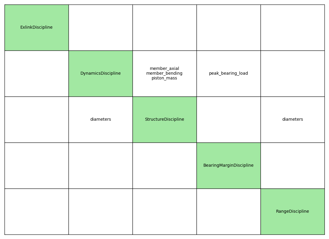
The N2 chart. Disciplines on the diagonal, couplings off it: above is feed-forward, below is feedback. Exactly one entry sits below the diagonal — StructureDiscipline returning diameters to DynamicsDiscipline, which sends back the member loads and the piston mass — and that pair is the fixed point (3.9). ExlinkDiscipline is worth noting for what is not in its row: it shares no variable with any other discipline, taking the design vector and returning \(\eta\), \(H\), \(B\) and the five geometric constraints straight to the optimizer.

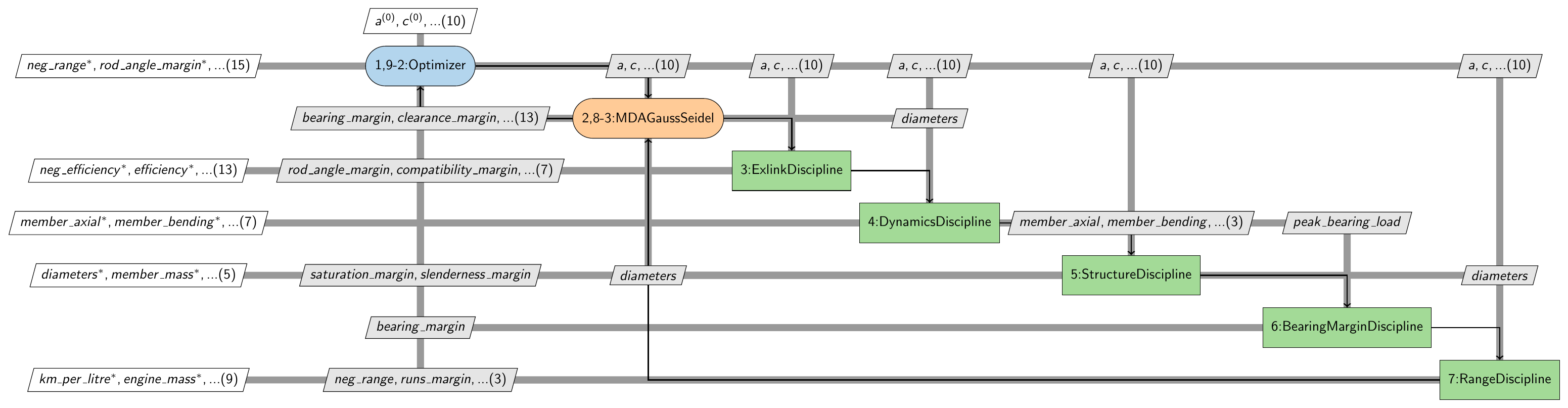
The XDSM: the same graph with the process on it. The optimizer runs steps 1 and 9-2, so it drives everything between; the Gauss–Seidel MDA runs 2 and 8-3, so it sweeps disciplines 3 to 5 and converges before anything downstream is evaluated. BearingMarginDiscipline and RangeDiscipline sit outside that loop because they consume the converged diameters and feed nothing back. That nesting is what MDF means: every point the optimizer sees is a self-consistent engine, paid for with one MDA per iterate. Ten design variables out, fifteen functions back.

method	module
sizing/dynamics fixed point (3.9)	exlink.coupled
the \(18\times18\) equilibrium solve	exlink.dynamics
yield / fatigue / buckling	exlink.sizing
forward mode and the envelope theorem (§4.2)	exlink.jacobian
derivatives through the MDA (§4.2)	exlink.dynamics_jacobian
MDF and the coupling measurement (§4.3)	exlink.formulations
bi-level outer approximation (§4.4)	exlink.minlp
the gear lattice (§4.4)	exlink.gears
tolerance and reliability (§4.5)	exlink.robustness
restarts on the manifold (§4.6)	exlink.scenarios
prescribed motion and range under every constraint (§4.7)	exlink.synthesis

The objective chain (3.3) is assembled in exlink.performance, which composes exlink.friction, exlink.mass_budget and exlink.vehicle and returns every intermediate, so a result can be interrogated rather than believed. Finite differences are still used where they are safe, and the boundary is deliberate: analytic for the extremum-based geometric quantities and for everything inside the MDA, differences for the clearance \(d\) (far from active), for \(\eta\), \(H\) and \(B\) (smooth, none tight) and for the range chain (one load solve, no fixed point, so eighteen columns is affordable).

4.9 Verification

Each discipline is checked against a result computed independently of it.

check	agreement
force chain against virtual work, \(M_r = -P\,\mathrm{d}\lambda/\mathrm{d}\theta_1\)	machine precision
torque integral against the \(p\)–\(V\) loop area	2 %
mean gas torque against mean total torque	\(10^{-6}\)
rigid-link invariants over the revolution	machine precision
joint reactions scaling as \(\Omega^2\) with gas load off	exact
slider-crank indicated efficiency against \(1-\varepsilon^{1-\gamma}\)	4 decimals
analytic Jacobians against converged central differences	\(\sim 10^{-6}\) relative
GEMSEO check_jacobian on the disciplines	passes
FORM system probability against 150 000 sampled builds	0.664 vs 0.665

Installation, the command line, the module map and a table mapping each result of §5 to the example that produces it are in Appendix B.