5. Results

Every number below is computed by the code of §4.8 and pinned by a test; none is transcribed. Speeds are quoted at the crankshaft, which turns twice per cycle on both mechanisms. Ranges are at one operating point with solid round members unless stated; §5.1 and §5.4 each re-score the principal comparison under one changed assumption and report their own pairs, which are not interchangeable with the headline.

Nine designs are referred to below and are collected here once.

design	range	what it is	feasible as specified
PUBLISHED_DESIGN	—	the historical baseline (§3.4)	no, five constraints
REFINED_DESIGN	—	geometric objective, augmented Lagrangian	yes
GRADIENT_DESIGN	—	geometric objective, SLSQP	yes
COUPLED_DESIGN	3338 km/L	minimum coupled mass; the strictly feasible reference	yes
RANGE_DESIGN	3388 km/L	range, constraints bound at the end	no, by \(1.5\times10^{-4}\)
range, constraints imposed	3501 km/L	(4.11) second form, nominal only	no, by \(2\times10^{-4}\)
RELIABLE_DESIGN	3395 km/L	(4.11) third form; the study’s result	no — relaxed spec
slider-crank, optimised	2888 km/L	the baseline of §5.4, over its own two freedoms	its own limits
slider-crank, capped	2467 km/L	the same, held to the linkage’s limits; §5.2 only	yes, on the cap

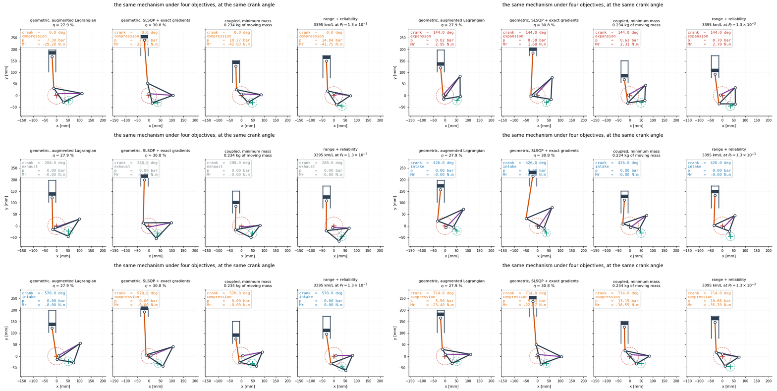
What each objective converged to from the same starting point, at one scale and one crank angle. Left to right: the geometric objective under an augmented Lagrangian and under SLSQP with exact gradients, then minimum coupled mass, then the study’s result. The two geometric optima are long-limbed and stand their cylinder high; the two that can see mass are visibly shorter and squatter.

5.1 The objective decides the design, and the quasi-static optimum is the worst place to be

Maximising the lever-arm measure (2.1) without inertia drives the design to \(W = 0.981\), a hair from the transmission-angle singularity, because that is where the quasi-static lever arm is longest. Restoring inertia makes that the worst available choice: shortening the swing rod moves the design off the singularity and buys half the bearing load, a smaller envelope and less than half the mass, at equal or better efficiency.

swing rod	\(W\)	\(\eta\)	\(H\) mm	moving mass	peak bearing
×1.00	0.9811	28.20 %	238.5	1.039 kg	12 629 N
×0.94	0.9670	27.79 %	227.8	0.610 kg	6 541 N
×0.88	0.9560	27.92 %	218.0	0.498 kg	6 647 N
×0.82	0.9488	28.56 %	213.2	0.450 kg	6 027 N

The proximity that lengthens the lever arm amplifies the accelerations: joint \(A\) sees 75 times the crank pin’s. Since \(m \sim (Ca)^3\) (§3.3) and every inertia load scales as \(\Omega^2\), structural mass grows as the sixth power of speed, and the quasi-static optimum admits no feasible structure above 2000 rev/min:

crankshaft speed	moving mass	peak bearing load
0 rev/min	0.25 kg	7.7 kN
2000	1.03 kg	12.5 kN
3000	8.43 kg	245 kN
4000	no section is thick enough

The effect is one of conditioning rather than of speed as such, and conditioning decides its sign. A well-conditioned slider-crank shows the opposite: its peak main-bearing load falls from 4735 N at rest to 2985 N at 4000 rev/min, because the peak gas force lands near top dead centre where the reciprocating inertia pulls the other way — classic inertia relief. Same physics, opposite sign.

The largest modelling conservatism does not repeal it

Solid round bars are the study’s most conspicuous simplification, and the natural guess is that the members are 30 % overweight. Both halves of that guess are wrong. The members are not where the mass is — 0.17 kg of a 12.9 kg engine, 1.3 %, against 10.13 kg of flywheel (78.3 %) — so thirty per cent of them is four grams. And boring them matters anyway, for a different reason. With RELIABLE_DESIGN unchanged and a bore ratio \(k = 0.6\):

crankshaft rev/min	solid km/L	tubular km/L	gain	members solid	tubular
1200	3206	3205	−0.0 %	123 g	134 g
1600	3350	3350	0.0 %	130 g	134 g
2000	3395	3411	+0.5 %	167 g	134 g
2400	3363	3423	+1.8 %	250 g	149 g
2800	3181	3385	+6.4 %	405 g	193 g
3200	2482	3249	+30.9 %	702 g	276 g

Nothing below the design speed, everything above it. The gas load does not change with speed and a bore does not reduce it, so at the bottom of the range a bore only forces the wall floor to grow the sections slightly. The inertia load is the member’s own mass times an acceleration proportional to \(\Omega^2\), and there a bore is compound interest: lighter members need less section, less section is lighter still, and the fixed point (3.9) converges somewhere else entirely. The tube is a conditioning improvement acting on precisely the mechanism this section is about.

It does not remove that mechanism. Sizing REFINED_DESIGN, which sits at \(W = 0.981\), the tube cuts the moving mass at 3000 rev/min from 8.34 kg to 2.66 kg and the peak bearing load from 244.8 kN to 74.2 kN — and at 4000 rev/min changes nothing at all, the design remaining unbuildable. A constant factor on member mass moves where the sixth-power divergence bites without removing it.

The bore ratio has an interior optimum, because a bored member has a wall and a wall has a minimum: at floor \(t = 1.5\) mm no member may be drawn below \(2t/(1-k)\), which is 6 mm at \(k = 0.5\) and 15 mm at \(k = 0.8\), and most of this linkage’s members are smaller than that when solid. Past some ratio the floor rather than the load sizes the light members. Optimising range over bore ratio and speed together lands at \(k = 0.579\) at 2276 rev/min for 3425 km/L against 3395 at 2000 — +0.9 % — with the engine at 10.4 kg rather than 12.9. Most of the improvement goes not into range but into being able to run 300 rev/min faster for the same range.

Two things generalise. A modelling conservatism was priced in the currency of the objective: “members 30 % lighter” was true and useless, “0.9 % of range, and only above the design speed” is a statement a decision can be made against. And the shape of the answer was not guessable from the conservatism, because in a coupled problem the size of an effect is not the size of the thing it acts on — anything reading the mass budget alone would have ruled tubes out. The model prices a tube through mass, stiffness and a wall floor and through nothing else: no local buckling, no end-fitting mass, no manufacturing cost. All three work against the tube, so +0.9 % is an upper bound.

5.2 The relaxation is a promise about tolerance

The requirements of §3.1 are a mathematical specification: eight numbers written down before any part existed. A tolerance study at IT8 says which of them this mechanism can hold. Only two are in question — the top-dead-centre gap \(g\) and the band each equality is relaxed into (3.11) — and the remaining five run from \(C_{pk} = 3.2\) to 493 and do not enter the discussion again.

constraint	nominal	\(\sigma\), first order	\(\sigma\), Monte Carlo	\(C_{pk}\)	violated
expansion_stroke	\(-0.04992\)	0.03645	0.02011	0.83	11.0 %
compression_ratio	\(-0.04998\)	0.00935	0.00516	3.23	0.0 %
rod_angle	\(-1.321\)	0.00556	0.00545	80.8	0.0 %
compatibility	\(-0.003854\)	\(4.0\times10^{-5}\)	\(4.2\times10^{-5}\)	30.7	0.0 %
tdc_gap	\(-0.004323\)	0.02173	0.01306	0.11	65.5 %
clearance	\(-47.65\)	0.03584	0.03221	493	0.0 %
side_load	\(-0.001414\)	\(4.3\times10^{-5}\)	\(4.1\times10^{-5}\)	11.5	0.0 %

tdc_gap has a standard deviation of 0.013 mm against a bound of 0.01 — the scatter is wider than the requirement — and expansion_stroke 0.036 mm against a half-band of 0.05. First order overestimates \(\sigma\) by up to 80 % here, so it is conservative rather than optimistic, which is worth stating because the opposite would make first-order robust design unusable in this region.

\(g\) is the most sensitive quantity in the problem, and four independent perturbations agree on its scale: IT8 machining gives \(\sigma = 0.013\) mm; snapping \(I\) 0.18 mm onto the gear lattice moves it from 0.003 to 0.058 mm; the minimum-norm equality projection moves it from 0.0009 to 0.0201 mm; and a crank-angle resolution below 360 samples errs by 44 %. A bound of 0.01 mm lies below every one — below the machining scatter, below the gear catalogue’s spacing, below the optimizer’s own convergence, and below the discretisation at which \(g\) is computed. It is not a requirement the rest of the model can resolve. A bound of 0.1 mm lies above all four.

What widening costs. The cycle feels \(g\) only through the volume trapped above the piston, and the clearance volume of 3000 mm³ is 3.73 mm of head space over a 32 mm bore. A 0.1 mm mismatch is \(+80.4\) mm³, so on one of its two revolutions the engine realises \(\varepsilon = 15.6\) rather than 16.0 and the reference design loses 0.47 % of range. That is the entire consequence of the relaxation, computed rather than argued. The bands are the same statement in other units: \(\varepsilon = 16 \pm 0.15\) is \(\pm 0.035\) mm of piston height, a shim under the head, and \(\mathrm{STE} = 74 \pm 0.15\) mm is \(\pm 0.2\) % of the stroke.

What widening buys. Evaluating (4.9) on COUPLED_DESIGN:

gap bound	band	system \(P_f\)	\(\beta\)	binding
0.010 mm	\(\pm 0.05\)	0.664	\(-0.42\)	tdc_gap
0.054 mm	\(\pm 0.05\)	0.329	0.44	stroke_lower
0.100 mm	\(\pm 0.05\)	0.328	0.44	stroke_lower
0.100 mm	\(\pm 0.12\)	\(1.0\times10^{-3}\)	3.09	stroke_lower
0.100 mm	\(\pm 0.15\)	\(1.9\times10^{-5}\)	4.12	stroke_lower

The second row is the useful one: once the gap is at 0.054 mm it stops binding, and no further widening of it changes anything. The bottom two rows differ from the third only in the band and span four orders of magnitude of failure probability. What sets the reliability of this mechanism is not the gap but how nearly the expansion stroke is required to equal 74 mm. Keeping the correlation works in the reassuring direction here — 0.664 against the 0.680 an independence assumption gives, converging to three figures by the last row — but what it costs is one matrix product and what it buys is that the number is a probability rather than a bound.

Most of that probability is avoidable, and free. The 0.664 is the price of ignoring the requirements while optimising rather than of the requirements themselves. Sampling 1200 designs about the reference and checking the best by reliability against the full constraint set gives a worst-case \(\beta_i\) of \(+0.610\) against \(+0.213\), a system \(P_f\) of 0.393 against 0.664 — a fall of 41 % — and a range of 3340 km/L against 3338, which is 0.05 % higher. All twenty-five of the best candidates are feasible. The deterministic optimum is dominated on both objectives at once, and the reliability is had for nothing rather than bought. This is the standard argument for RBDO, measured rather than asserted: a deterministic optimizer converges onto its active constraints because nothing in the formulation rewards standing off them, and a design sitting exactly on \(g = 0\) fails half the time.

The effect is not peculiar to this linkage. Optimising the conventional baseline under the linkage’s rod-angle and side-load caps — a specification it has no reason to meet, imposed only so that it has an active constraint to converge onto — it converges onto it, at \(\gamma = 0.02000\) against a bound of 0.02, with \(P_f = 0.595\). Three builds in five miss the requirement. Giving up 0.4 % of the obliquity, to \(r/l = 0.09580\), costs 0.17 % of range and takes the failure probability to \(9\times10^{-9}\). Two toleranced dimensions instead of eleven, two design variables instead of ten, a different topology and a different optimizer, and the same shape of result: the effect belongs to deterministic optimization under tolerance, not to this mechanism.

The transferable statement is about the order of the two studies. The bounds were fixed first and the tolerance study run on the result, and by then the specification contained one requirement finer than the model’s own resolution and one that governed the reliability of everything else — neither visible in any nominal quantity. Running the tolerance study against the specification, before any design exists, costs one Jacobian and answers a question the optimizer never asks: which of these numbers the specification is entitled to contain.

5.3 The reliability model failed twice, in different places

Every probability above is first order, over an uncertain vector containing only the eleven dimensions. Both restrictions were stated as limitations when they were adopted (§4.5). Testing each found an error, and the two are independent.

The uncertain vector was too narrow, and the omission decided the design

Widening the vector to seventeen — adding yield strength, ultimate strength, stiffness, density, the friction coefficient and the explosion ratio that sets the gas load — changes nothing that was already priced. All eight geometric constraints are 100 % dimensional to the last figure reported, exactly rather than approximately: the widened model takes those rows from the same analytic Jacobian rather than differencing them, so a disagreement would have been physics rather than a step size.

What was not priced decides the design. The system probability goes from \(9.4\times10^{-3}\) to \(5.0\times10^{-1}\), and all of it is one constraint:

constraint	\(\beta\)	dominant source of its variance
saturation	460	explosion ratio, 87 %
slenderness	63	ultimate strength, 94 %
bearing	36	explosion ratio, 100 %
runs	26	friction 51 %, explosion ratio 49 %
gear	0.00	explosion ratio 71 %, yield strength 29 %

The gear pair the mixed-integer master picked — \(m = 0.8\), \(z = 48\) — sits exactly on its face-width limit, at 11.99997 against a bound of 12. Whether it fits is a coin flip. The narrow model could not have found this, and not through carelessness: the face width is not a function of any of the eleven dimensions but of the torque transmitted and the strength of what the pair is cut from, so a tolerance study on lengths and angles has nothing to say about it however finely those lengths are held.

The fix costs nothing. Re-scoring RELIABLE_DESIGN on the three candidate pairs, the ordering is the same on every column: the pinned pair is the shortest ranged (3394.9 km/L), the heaviest (12.94 kg) and the only one whose gear constraint binds, while \(m = 1.0,\ z = 39\) gives 3395.3 km/L at 12.91 kg and recovers the geometric probability exactly. There is no trade to negotiate — the pinned choice was worse on all three counts, and a range gap of 0.03 % was far too small to have revealed it. The study’s result should not be built with the pair the master returned.

Two entries in the variance split are worth reading. slenderness rides almost entirely on the ultimate strength rather than the yield, which says the members are sized by fatigue: the endurance limit is \(0.5 S_u\) before Marin corrections, so the scatter that matters is in \(S_u\). And runs splits evenly between friction and gas load, which is the mechanical efficiency of §5.4 restated as a variance — the margin between indicated and brake work is a difference of two uncertain quantities of comparable size. Stiffness and density earn their place by not mattering, 0 % and 6 % of one constraint between them.

The general shape is not about gears: a reliability model prices what its uncertain vector contains and reports silence as safety on everything outside it, and the constraint that governs a design has no obligation to be inside. §4.5’s honest statement that only seven constraints could carry a probability was true, correctly worded, and read as a footnote rather than as the warning it was.

The estimate was linearised at a kink

150 000 exact builds drawn from the same covariance, each analysed in full, do not agree with FORM:

design	specification	FORM	sampled, 150 000 builds	ratio
COUPLED_DESIGN	as written	0.6454	\(0.6650 \pm 0.0012\)	0.97
RELIABLE_DESIGN	§5.2’s bounds	\(1.35\times10^{-3}\)	\((9.28 \pm 0.25)\times10^{-3}\)	0.145

FORM is accurate on one design and optimistic by a factor of seven on the other, and the difference between them is the whole finding. The expansion stroke is \(\mathrm{STE} = \max(\lambda_{tdc,1}, \lambda_{tdc,2}) - \min\lambda\), the stroke being measured from the higher of the two top dead centres because that is the one setting the clearance volume. A maximum of two smooth functions is not smooth at the tie, and linearising it uses whichever branch attains it at the nominal design. COUPLED_DESIGN has its two top dead centres 6.97 µm apart, comfortably more than the scatter can bridge. RELIABLE_DESIGN has them 0.107 µm apart — and has them there because driving the gap to zero is exactly what its own \(g\) constraint rewards. The parts, whose dimensions scatter by some 7 µm, straddle that tie in every single build.

Measuring the branches separately settles it. The stroke from TDC 1 has \(\sigma = 0.01814\) analytic against 0.01817 sampled, skew \(-0.01\), \(\beta = 3.00\); from TDC 2, 0.02304 against 0.02306, skew \(-0.02\), \(\beta = 2.36\); the maximum of the two has \(\sigma = 0.02016\) and skew \(+0.11\). Each branch is Gaussian to two decimal places in its skew, so FORM is exactly right on either one. What it did was linearise branch 1, which attains the maximum by a tenth of a micron and is 27 % less sensitive than branch 2. The parts breach branch 2. The estimator was never wrong; the formulation was, presenting a maximum as a single differentiable function and handing the linearisation the branch that happened to be on top.

The fix is one extra Jacobian row: carry both branches as separate constraints. For the upper bounds this is exactly right rather than merely safe — the realised stroke exceeds its bound when either branch does, which is a union over correlated normals, and a union over correlated normals is precisely what the orthant integral already computes. With that change FORM gives 0.6636 against 0.6650 sampled on COUPLED_DESIGN (0.2 %) and \(9.38\times10^{-3}\) against \(9.28\times10^{-3}\) on RELIABLE_DESIGN (1.1 %). No sampling, no second derivatives, no extra analyses.

Second derivatives are the wrong instrument, and the wrongness is measurable. Curvature is the natural first guess. Differencing the analytic gradient — the well-conditioned route to a Hessian, the first derivatives being exact — separates the maximum from its branches. On the maximum, \(\lVert\nabla^2 g\rVert \times h\) is constant at 0.003283 to five significant figures across a fiftyfold range of steps and the matrix is 100 % asymmetric at every one: a fixed jump in the gradient divided by a shrinking step, which is to say there is no second derivative there to find. On a single branch the norm is constant at \(10^{-5}\), the matrix is exactly symmetric, and the value is five orders of magnitude smaller — a genuine second derivative, and a negligible one. The jump is the branch switch: perturbing \(a\) by 0.3 µm moves \(\partial\mathrm{STE}/\partial a\) from 0.0093 to 0.52, a factor of 56. The constraint surface is not curved but kinked, and no order of Taylor expansion repairs a kink. What was needed was not a second derivative but a first one, of the other branch.

Three things generalise. A sampling check is a control rather than a refinement: nothing in the FORM output — not the index, not the correlation, not the per-constraint breakdown — carried any sign that the estimate was wrong, because from inside the linearisation it was self-consistent. Optimisation drives designs onto the non-smooth features of their own constraints: the tie was not bad luck but the direct consequence of an objective that rewards a small gap, so any deterministic optimum should be suspected of sitting on whatever non-smoothness its formulation contains. And diagnosis beat correction: second derivatives would have cost eleven extra Jacobian evaluations per design point and produced noise, while finding out why the estimate was wrong cost one sampling run and produced a fix that is exact, free, and applies at every design rather than only the one checked.

5.4 The topology is worth 17.6 %, and the dimension count is not the reason

Both engines complete their four strokes in 720° of the shaft power is taken from, at the same compression ratio, the same clearance volume and the same fuel per cycle, sized by identical structural and tribological code. Both are optimised — the baseline over the two freedoms it has, rod obliquity and speed.

	slider-crank, optimised	EX-link (RELIABLE_DESIGN)
\(r/l\)	0.195	—
crankshaft speed	2151 rev/min	2000 rev/min
power strokes per minute	1076	1000
indicated efficiency	0.457	0.480
mechanical efficiency	0.787	0.865
brake efficiency	0.359	0.416
engine mass	16.9 kg	12.9 kg
range	2888 km/L	3395 km/L

+17.6 %, and that is the whole comparison: there is no firing-rate correction to make, because taking power off the shaft that turns twice per cycle leaves both engines with the same relation between speed and cycles, and no speed mismatch to argue about, because re-scoring the baseline at 2000 rev/min gives 2883 km/L and moves the figure to +17.8 %. Against COUPLED_DESIGN rather than the study’s result the same comparison gives +15.6 %.

The linkage is ahead on all three terms at once, and the three come from different physics: indicated efficiency from expansion through 20.8 volumes against 16.0; mechanical efficiency from 9.7° of rod angle against 11.2° and a side-load ratio of 0.018 against 0.039; and mass from a flatter torque curve needing less flywheel. The thermodynamic term — the feature the topology exists for — is the smallest of the three, five per cent of indicated efficiency.

The advantage is not a dimension count

The obvious explanation of the other two terms is that the linkage has eleven dimensions to place and the slider-crank two. That explanation is testable without inventing a third topology: give the conventional engine a third freedom. The wrist-pin offset is the cheapest one a real engine has, and optimised over its own variables at the same compression ratio through the same code it moves the design from \(r/l = 0.1954\) to 0.1943 at \(d/r = +0.156\), the mechanical efficiency from 0.7867 to 0.7921, the mass from 16.93 to 16.84 kg, and the range from 2887.7 to 2902.5 km/L — +0.51 %.

Taken literally, the dimension-counting explanation predicts badly: nine such freedoms extrapolate to about 4.6 % against the 17.6 % the linkage reaches, an under-prediction by a factor of nearly four. What the offset does is instructive precisely because it is so narrow. It rearranges the side load, so mechanical efficiency improves and mass follows slightly. It cannot touch the indicated efficiency, because the piston still makes two identical strokes per revolution however far the pin is moved — there is no extended expansion to be had from a slider-crank at any number of dimensions — and it cannot touch the flywheel, because there is no half-speed shaft to hang one on. The eleven dimensions are what let the linkage exploit its topology, not what give it the advantage. Two topologies still establish a contrast; a genuine third — one carrying its own internal 2:1 ratio, which is what unequal strokes require — would be needed to make it a trend.

Over a schedule the advantage widens to 19.3 %

An optimum found at one speed may be an artefact of the speed. Scoring both designs over a four-point schedule spanning 0.8 to 1.4 times the design speed, as one engine rather than as one engine per point:

crankshaft rev/min	share	EX-link km/L	slider-crank km/L
1600	0.20	3347	2811
2000	0.40	3315	2772
2400	0.25	3243	2705
2800	0.15	3046	2589
cycle		3260	2733
worst / best		0.910	0.921
one engine		18.85 kg	29.53 kg
of which flywheel		15.84 kg	28.29 kg

Neither design was tuned for the schedule. The EX-link gives up 4.0 % of its single-point range and the slider-crank 5.4 % of its own, so the advantage widens from +17.6 % to +19.3 %.

Two modelling points carry that result. The aggregation is a distance-weighted harmonic mean, \(1/R = \sum_i w_i/R_i\), because the figure of merit is distance per unit fuel and it is fuel per unit distance that adds; an arithmetic mean flatters a design whose range collapses at one point, and catching exactly that is what a schedule is for. And one engine must satisfy every point, with the two ends of the schedule sizing different parts in opposite directions: the fastest point sizes the structure, every inertia load growing as \(\omega^2\), while the slowest sizes the flywheel, the inertia needed to hold a given speed fluctuation going as \(\omega^{-2}\). Composing the two is exact rather than conservative here, the flywheel being concentric with its shaft and so adding no inertia force. The composition is the whole of the 4.0 %: the EX-link’s structure at 2800 rev/min is 3.0 kg against 2.8 at the design point, while its flywheel goes from 10.1 to 15.8 kg. An engine specified over a range of speeds is a flywheel problem.

The gap widens not because the flywheel advantage grows — the two wheels stand in a fixed ratio of 1.79 at every speed, both scaling as \(\omega^{-2}\) from torque curves whose shapes do not move — but because the mix changes. The slider-crank is the lighter mechanism, two members and no gear pair against a trigonal link, a rocker and a gear pair, and the heavier engine, because the item it loses on is the flywheel and the flywheel is most of both engines. Widening the speed range takes the flywheel from 78 % to 84 % of the linkage’s mass and from 92 % to 96 % of the baseline’s, weighting the comparison further towards the one item the EX-link wins by 1.79, and the total-mass ratio moves from 1.31 at a point to 1.57 over the schedule. The wider the speed range an engine must cover, the more of its mass is flywheel, and the more a flat torque curve is worth.

The baseline was given its remaining freedom back: re-optimising \(r/l\) against the schedule moves it from 0.195 to 0.198 and the cycle range from 2733.2 to 2733.7 km/L, four parts in ten thousand — its point optimum was already its cycle optimum. The EX-link was not re-optimised over the schedule, which would be an eleven-variable solve, so +19.3 % is a lower bound on what a cycle-aware design would reach. The weights themselves are an assumption; without a surveyed track there is no defensible way to derive them. What the schedule establishes is not a more accurate range but the absence of an artefact.

Two conservatisms, both running the same way

No gas exchange is modelled. Both cycles hold intake and exhaust at plenum pressure, so neither engine pays any pumping work, which sounds even-handed and is not. An over-expanded engine opens its exhaust valve on a charge that has expanded further and therefore sits closer to ambient: \(p/p_0 = 1.23\) for the EX-link against 1.70 for the slider-crank, and the work still recoverable by isentropic expansion to ambient — the theoretical maximum, not an achievable figure — is 9.5 % of indicated work against 26.4 %. The model discards both, removing a loss roughly two and a half times larger for the conventional engine. Separately, the baseline is allowed to violate the 10° rod-angle and 0.02 side-load caps the linkage is held to, which come from the linkage’s own brief and which practical slider-cranks exceed routinely. Both conservatisms run against the linkage, so 17.6 % is a lower bound on both accounts.

One runs the other way, and is why the mass column is not quite like-for-like: the baseline carries a flywheel sized for a single-cylinder four-stroke’s turning-moment diagram, the worst case in this class. Both flywheels are sized by the same rule at their own shaft speeds, so the comparison is at least consistent. Giving both engines tubular members and re-optimising each moves the baseline to 2929 km/L and the linkage to 3425, narrowing the comparison from +17.6 % to +17.0 % — the bore helping the conventional engine marginally more, its two members being a larger share of a smaller mechanism.

5.5 The announced problem, solved, and where the search must be helped

Problem (4.11) is: maximise range, hold every constraint, constrain a system probability of failure. Solving that needs the bounds §5.2 identifies, because at the bounds as written no design reaches the target. The run used the gap at 0.054 mm and both bands at \(\pm 0.15\):

	start (COUPLED_DESIGN)	result (RELIABLE_DESIGN)
range	3338 km/L	3395 km/L
worst constraint	—	\(-2.2\times10^{-7}\)
system \(\beta\) as the solve measured it	3.08	3.00, on its target
system \(\beta\) as §5.3 corrects it	4.12	2.35
system \(P_f\), corrected	\(1.9\times10^{-5}\)	\(9.4\times10^{-3}\)

1352 evaluations, 61 minutes, the iteration cap reached rather than a convergence test. The two \(\beta\) rows are the important part and the second is the one to believe, being confirmed against 150 000 exact builds at \(9.28\times10^{-3}\). The solve did hold its target — on the constraint set it was given, which linearised the expansion stroke on the branch that attains the maximum, while it is the other branch the parts breach. Two things follow and they pull apart. The range is unaffected: 3395 km/L is a measurement of the design rather than of the estimator, and every figure in §5.4 stands. What does not stand is the claim that this design meets a reliability requirement.

Only the band matters to that. Re-scoring the same design against the 0.1 mm gap gives \(P_f = 9.382\times10^{-3}\) against \(9.393\times10^{-3}\) at 0.054 mm, because the gap sits at \(\beta = 8.1\) either way; the band is a different matter, the design being inadmissible at \(\pm 0.05\), reaching \(\beta = 0.19\) at \(\pm 0.12\) and 4.53 at \(\pm 0.20\). Two constraints are active in the reliability sense — stroke_upper_2 at \(\beta = 2.36\) and stroke_upper_1 at 3.00 — and they are the same requirement measured from the two top dead centres, which is the whole of §5.3. The next is ratio_upper_2 at 5.14 and everything below is a spectator, which is otherwise the shape a reliability-constrained optimum should have. Imposing the constraints without the reliability requirement reaches 3501 km/L, 3 % more, by converging onto its active constraints: the 3 % is the price of standing off the boundary, and the two figures answer different questions.

Re-solved on the corrected constraint set. From COUPLED_DESIGN with branch-aware constraints and a 200-iteration budget — 2633 evaluations, 5 h 45 min — the result reaches 3399.2 km/L at \(P_f = 4.1\times10^{-3}\) (\(\beta = 2.64\)) and 13.43 kg, dominating the shipped result on both objectives for half a kilogram. Three things about it are worth more than the numbers.

It did exactly what it was told, which is not the same as meeting the target. The search steers on \(\min_i\beta_i\) (§4.7) and drove three constraints there simultaneously — stroke_upper_1 at 3.003, ratio_upper_2 at 3.005, ratio_upper_1 at 3.042 — so the steered quantity is met to three decimals while the system index sits at 2.64, the union of three constraints each at \(\beta = 3\) being likelier to be missed than any one. That is the inequality of §4.5 made visible as a 0.36 discrepancy, and it widens with better convergence, because a better-converged optimum pushes more constraints onto the boundary.

The design left the kink of its own accord. Its top-dead-centre gap is 0.016 mm rather than \(1.07\times10^{-4}\), two orders of magnitude clear of the tie. Nothing asked it to move: with both stroke branches priced, collapsing the two top dead centres no longer buys anything. The formulation that made the estimate correct also removed the incentive that had put the design where the estimate was wrong.

It still stopped at the cap. 3399 km/L is a lower bound as 3395 was. What the re-solve settles is that the cap is not hiding much — nearly six hours of extra budget bought 0.13 % of range — and what it does not settle is where the formulation tops out. For that reason it is reported rather than adopted: promoting an unconverged result to be the study’s answer, and redrawing every figure from it, would trade a documented lower bound for an undocumented one.

Where the search has to be helped, and where it does not. Two instruments were built for two obstructions. One removes its obstruction; the other turns out not to have one, and a method that was not needed is as much a result as a method that was.

Manifold-projected restarts reach feasibility in 0 of 6 attempts on the range problem, which is why the multistart of §4.6 is inconclusive there — not that the restarts found worse optima but that they never found the feasible set. Six starts drawn the same way, 5 % scatter about COUPLED_DESIGN, put through the epigraph problem \(\max_{X,t} t\) subject to \(c_i(X) \ge t\), go from 0 of 6 feasible to 6 of 6 at about 290 evaluations each, 42 minutes in total. It works where the range solve does not because it has no objective to trade against the constraints, so every constraint pulls the same way and its QP always has somewhere to go; starts as far as 14.9 outside restore no more slowly than starts 1.5 outside. The restored points are inside and barely, with margins between \(2.4\times10^{-3}\) and \(7.8\times10^{-3}\) — which is what the thinness of §4.1 means in practice, and is enough for a gradient method to start from without being enough to call a design robust. What has not been measured is the second half: six restored starts make the multistart answerable, and answering it needs six range solves from them, at six times the cost of the run above.

A continuation in \(\beta\), warm-starting each rung from the last, is the natural instrument for the other obstruction — that SLSQP with a reliability target attached returns its starting point unchanged. Measured against a single solve at the same iteration budget from RANGE_DESIGN, the ladder of five rungs at 30 iterations costs 2060 evaluations against 1435 and ends at \(\min_i\beta_i = 2.651\) against the single solve’s 3.000. The rungs behave as designed — each moves, and the climb is monotone in reliability from \(\beta = 0.001\) to 2.651 while the range rises from 3388 to 3402 km/L — but thirty iterations is not enough for any rung to converge, so the budget is spent restarting rather than arriving. The reason is not that continuation is a bad instrument but that the obstruction it was built for is absent: the non-movement was measured under the first form of (4.11), with the coupled and vehicle constraints bound only at the end, and under the second form with the branch-aware constraint set the search moves freely from the same start and reaches its target unaided. Given a search that can move, subdividing its target only fragments its budget. The fault was in the constraint set, and one extra Jacobian row did more for reachability than a homotopy does.

5.6 Asking for the topology instead of supplying one

§5.4 measures a topology that was given. This section removes that, and applies the second family of §2.2 — the spring-connected model — to the question the engine poses: turn the circular motion of one input shaft into the piston motion an extended-expansion cycle needs.

The design domain holds eight nodes and twelve candidate members: the input shaft grounded at the origin with its pin, a second grounded shaft carrying a pin at twice the input speed and the opposite sense — the relation a 2:1 gear pair imposes, which the search may use or leave out — a spare grounded pivot, two free nodes, and the piston on the cylinder axis. Each candidate member is a spring whose presence is a design variable, penalised towards rigid or absent, giving 26 variables in all. The target is \(\lambda^\star(\theta_1)\) from §3.5’s requirements: two equal maxima and two unequal minima, \(\mathrm{STE} = 74\) mm and \(\varepsilon = 16\) exactly. Six random starts were walked up a four-rung penalisation schedule and then rounded to a discrete linkage; five completed inside a 50-minute cap and one did not.

start	rms [mm]	strain	members	first harmonic	second	four phases	STE	STC
2	37.00	\(1.4\times10^{-6}\)	2	29.32	7.43	no	—	—
3	7.19	\(5.8\times10^{-7}\)	3	0.0000	36.89	yes	73.775	73.775
5	21.43	\(7.9\times10^{-6}\)	2	19.79	21.04	no	—	—
6	29.38	\(7.5\times10^{-5}\)	1	27.12	33.85	no†	—	—
7	28.61	\(6.2\times10^{-7}\)	4	36.77	3.42	no	—	—
1	cap reached at rms 5.93, still undecided

The target’s own harmonics are 9.02 mm at the first and 32.33 mm at the second, and its standard deviation — the score for producing no useful motion at all — is 23.74 mm. † Start 6 is not a mechanism at all: the mobility test of §5.7 reads \(4.3\times10^{-2}\) on it against exactly zero for every other row, so its single element leaves the piston undetermined. The conclusion below is unaffected, but the diagnosis is.

The method works and produces real linkages. Every completed start returned a discrete mechanism running at a strain of \(10^{-7}\) to \(10^{-5}\), which is the stiffness floor: the springs are standing in for rigid links rather than deforming. Nothing about the topology was assumed, and the search chose its own member count, from one to four.

Not one of them is an extended-expansion mechanism. One start reached a clean four-stroke motion, and it is an Otto engine: \(\mathrm{STE}\) and \(\mathrm{STC}\) equal to six figures, with an asymmetry of zero rather than the 18 mm the specification needs. What it built is a slider-crank hung on the geared shaft — one rod from that shaft’s pin to the piston — with the input shaft carrying a two-bar chain that reaches nothing.

The failure is an identity, not a numerical accident. Reach the piston from the geared shaft alone and its height is a function of that shaft’s angle, \(-2\theta_1 + \varphi\); every term is then periodic in \(\theta_1\) with period \(\pi\), so every odd harmonic vanishes exactly. The two up-and-downs are there and the two halves of the revolution are identical, which is precisely a plain four-stroke Otto motion. Measured on that design the first harmonic is \(1.5\times10^{-5}\) mm against a second of 36.89 — seven orders of magnitude down, and the residue is the equilibrium solver’s precision rather than physics. The opposite degeneracy also appeared: start 7 reaches the piston from the input shaft alone, so its motion is periodic in \(2\pi\), gives one up-and-down per revolution, and is not a four-stroke at all.

So the asymmetry lives entirely in the first harmonic, and the first harmonic requires both shafts. This is what EXlink’s trigonal link is: a single body whose three corners take the swing rod from the half-speed shaft, the crank from the fast shaft, and the piston rod. Read that way it is not a construction detail but the feature the topology exists for, and a synthesis that never joins the two chains cannot produce extended expansion however well it fits everything else.

Why the search stops where it does. The second harmonic carries 32.33 mm of the target’s 33.6 mm of harmonic amplitude, so a design that captures it alone has already taken most of the objective: 7.19 mm of error against the 23.74 mm of doing nothing. The missing first harmonic is worth only 6.38 mm of rms — and it is unreachable by descent, because the two-bar chain the search kept touches nothing that reaches the piston, so the objective is flat in its geometry. Differencing at the answer gives a gradient of at most \(1.5\times10^{-4}\) over that chain’s six geometry variables against 1.69 over the six that drive the piston: four orders of magnitude. It is the failure of Appendix C §C.7 in a new place — a gradient method stalls where the quantity of interest does not vary — and here it is the topology that would have to change first, which no amount of geometry descent will do.

Two faults in the formulation were found by running it, and both are worth recording because neither is visible in a statement of the method. The first: a member-count term of 1 mm made “build nothing” a strict local minimum, since a piston connected to nothing scores the target’s standard deviation and pays no count, and one start duly converged to it — fully discrete, and a mechanism with no members. The repair is a floor on the delivered stroke, which charges a static piston twice the required travel. The second: a strain weight of 50 mm let a design fit the target to 2.0 mm while carrying 3 % strain, so the search was being paid to leave members half present — a half-stiff member lets an overconstrained network move by giving rather than by articulating. That answer fitted well and rounded to nothing. Raising the weight to 800 mm and ramping an explicit discreteness charge alongside the penalty exponent took the resolved designs from a discreteness of 0.43 to 0.02.

What this establishes and what it does not. It establishes that the piston must be reached from both shafts, by an argument that is exact rather than empirical, and it demonstrates the method end to end on this problem — ground structure, continuation, rounding, and a mechanism at the end of it. It does not establish that no alternative topology exists. Twelve candidate members and six starts is a small search next to the published spring-connected studies, which use far larger domains and many more starts; a domain that offered a three-corner body directly, rather than requiring the search to assemble one from binary members, would be the obvious next step. And the objective here is kinematic, so even a success would have produced a candidate rather than a design: the range chain of §3.3 is what would decide whether it beat 3395 km/L.

5.7 Giving the synthesis more freedom, and what it exposes

§5.6 concludes that extended expansion needs the piston reached from both shafts, and leaves two obvious objections: the domain offered no three-cornered body, so the linkage that does the joining could only be assembled from bars that are individually useless; and the 2:1 relation was given rather than chosen, so the run could not say whether a synthesis wants one. Three changes answer both.

Every shaft now carries its own angle as a coordinate of the equilibrium, prescribed only for the input. Candidate gear pairs drive them, one presence per (pair, ratio) over a catalogue of 1, 2, 3 and 4 to one — whole numbers because the cycle has to close, a shaft turning \(r\) times per input revolution returning to its start only when \(r\) is an integer. A pair meshes externally, so its pitch radii are read off the centres the search chose, \(r_i = dr/(1+r)\) and \(r_j = d/(1+r)\), and it costs the slip at the pitch point, \(\tfrac12 k(\rho)(r_i\vartheta_i + r_j\vartheta_j - \varphi)^2\); writing it as slip rather than as an angular error is what makes the mesh consistent for free, with no separate centre-distance constraint. And ten candidate bodies join the twelve bars — rigid triangles carried as three springs sharing one presence, so a three-cornered link switches on as a unit.

The domain grows from 26 design variables to 45. Verified independently: a fitted pair holds its ratio to the solver’s precision and delivers exactly \(r\) up-and-downs per input revolution, its radii summing to the centre distance; a switched-on body holds all three sides; and the bars-only domain remains a special case of the same solver, still reproducing the slider-crank’s closed form to \(4.3\times10^{-5}\) mm.

start	rms [mm]	strain	slack	elements	gear	first harmonic	second	verdict
1	23.74	\(1.9\times10^{-5}\)	0	5	none	0.001	0.001	detached from the input
2	46.06	\(1.3\times10^{-5}\)	0	3	2:1	0.000	44.12	Otto, STE = STC = 88.401
3	46.41	\(5.9\times10^{-4}\)	0.71	2	none	59.12	7.92	not a mechanism

Six starts were run on the same seeds as §5.6, and three completed inside a 90-minute cap: the enriched domain costs about 13 s a gradient against 3.6 s, and the three that did not finish were still on their second or third rung. That is itself worth recording — freedom is not free, and 45 variables under finite differences is close to the limit of what this objective can be searched at.

The search chooses two to one. Offered four ratios and the option of none, the starts that kept a pair kept 2:1 — the only integer ratio that gives a four-stroke from the geared shaft. That is the one thing §5.6 was handed and could not test, and it comes back the same.

A body was used, and it was not enough. Start 2 is the sharpest result here: fully resolved, running at a strain of \(1.3\times10^{-5}\), holding a 2:1 pair and two three-cornered bodies — and still an Otto engine, with the two strokes equal to six figures. The reason is visible in its element list, P2-F1, P2-F1-F2, P2-F1-S: every one of them hangs off the geared shaft’s pin and not one touches the input’s. So supplying the body removed the barrier §5.6 measured without removing the outcome: a three-cornered link whose corners all come from the same chain is still a one-shaft mechanism, and the identity applies to it unchanged. What extended expansion needs is not a body but a body that bridges — which is exactly what EXlink’s trigonal link does, and a sharper statement than §5.6 could make.

The extra freedom brought two failures the smaller domain could not have.

Disconnection. Start 1 resolved to five elements, none of which touches a driven node: a mechanism detached from the input, with a piston that does not move. The travel floor charges it twice the required stroke and it still cannot escape, because SIMP flattens the gradient near \(\rho = 0\) — the void is a broad flat basin, and once a design drifts in there is nothing to climb.

Under-constraint, which is the one that lies. Start 3 reported extended expansion: four monotone phases, an asymmetry of 70.9 mm, a first harmonic of 59.1. It is not a mechanism. It kept no gear, so the geared shaft’s angle is a coordinate nothing resists, and where such a design goes is chosen by the solver’s ridge and its warm start rather than by the linkage. Strain does not see this — a loose mechanism strains nothing — so the reading has to come from the other side: the largest component the piston’s coordinate has in the null space of the reduced Hessian. It is \(0.71\) there, against exactly zero at every genuine answer in this study, §5.6’s included.

Then the domain was checked, and the objective turned out to be at fault. A negative result from a search means nothing until the domain is shown to contain the thing being looked for, so EXlink itself was written into it: three candidates and a pair — the swing rod P1-F1, the trigonal link as a body P2-F1-F2, the piston rod F2-S, and a two-to-one mesh. The spring model reproduces its analytic kinematics to \(6\times10^{-3}\) mm, at a strain of \(2.3\times10^{-5}\) and no slack, and scores it correctly: STE 74.09 mm, STC 56.39 mm, an asymmetry of 17.70 mm, \(\varepsilon = 16.12\). The domain was never the problem. Every corner is a design variable — the two free nodes are the trigonal link’s own corners, and the body’s three sides follow from where they are put — so nothing about its shape was fixed in advance.

What was at fault was the comparison. Where \(\theta_1 = 0\) sits is a choice, not a property of a mechanism: rotate a design about its input axis and every crank phase moves with it, giving the same engine with its cycle starting elsewhere. Scoring against the target at a fixed datum charges for that, and it charges enough to invert the ranking:

design	as posed	with the datum free	best shift
EXlink itself	13.97 mm	4.05 mm	170°
§5.6’s best (Otto)	7.19 mm	7.19 mm	0°
§5.7’s best (Otto)	46.06 mm	10.67 mm	123°

The degenerate answers had tuned their phase to the datum and the real mechanism had not, so the objective preferred an Otto engine to the engine being searched for — 7.19 against 13.97 — and no amount of searching could have recovered from that. A harmonic coefficient carries a phase too, and a rotation by \(s\) turns the \(n\)-th of them by \(ns\), so the harmonic term was charging an order-one error per harmonic for the same non-quantity. Profiling the datum out — one transform pair, since minimising the squared difference over the shift is maximising the circular cross-correlation — puts the full objective at 7.53 for EXlink against 21.18 and 26.87 for the two searches’ best, which is the ordering a synthesis needs before it can be said to have searched at all.

That is the honest account of §5.6 and §5.7 as first run: the identity they establish stands, and the domain is adequate, but the ranking they were searching under was wrong.

That last point is the transferable one, and it is a property of the method rather than of this engine. Strain catches an over-constrained answer; nothing in the standard formulation catches an under-constrained one, and an under-constrained answer can report any motion at all — including the one being searched for. It appeared here only because shaft angles became coordinates, and every enrichment of a spring-connected domain has the same exposure: more freedom means more ways for the equilibrium to stop determining the output. A mobility test belongs beside the strain test in any such run, and re-reading §5.6’s starts through it reclassifies one of them.

The three repairs

What was missing was not freedom but conditions on it, and the datum. All three are now in the formulation.

The datum is profiled out, as above, so a mechanism is no longer charged for where its cycle happens to start.

Mobility is charged. :attr:~exlink.topology.Motion.output_slack was already being computed as a diagnostic; it is now a term. An answer the equilibrium does not determine costs 200 mm per unit of slack, which prices start 3’s 0.71 out of contention rather than leaving it to be caught by a reader.

Bridging is charged, and this is the one that needed care. §5.6 derives – it does not assume – that a piston reached from one shaft alone has every odd harmonic identically zero, so extended expansion requires both driven pins joined to the piston through the linkage. Imposing a proven necessary condition is not assuming the answer: nothing in it says how the two chains meet, how many elements it takes, or what shape the body that joins them has. The measure is a bottleneck path on the graph the presences describe – the value of a route is its weakest presence, the value of a pin is its best route – which gives 1 for a fully built chain, 0 for none, and the weakest link for a half-built one, so it is something a gradient can climb rather than a yes-or-no test.

A pin’s reach is then gated by how far its shaft is actually driven, and that gate is not decoration. Without it the condition is satisfiable vacuously: a shaft carrying no gear is a passive grounded pivot, so joining the piston to its pin carries no second source of motion, and a run duly reached 1.00 on both pins while keeping no pair at all. Dropping the pair from EXlink’s own linkage takes its reach from (1.00, 1.00) to (1.00, 0.00) and its objective from 7.54 to 215.59. §5.6’s domain prescribes both shaft speeds and has no gear element, so the gate is inert there and its figures stay comparable. A fourth guard came out of the results in the same way: an answer must deliver the stroke. A piston wobbling by two millimetres can show four monotone phases and an asymmetry above one, and start 3 did — harmonics of 1.9 and 2.5 mm, travel of 7.1 against a required 74 — and was reported as extended expansion until the size of a motion was tested alongside its shape.

A fourth change is not a condition but a scale. The bounds are deliberately loose because the answer is not known in advance; a start drawn that loosely is a different thing, and the first runs drew nodes over half a metre apart and elements three hundred millimetres long for a piston that travels 74. Starts are now drawn on the specification’s own scale, a stroke and a half, which says nothing about shape.

Together these rank the designs the way a synthesis needs before it can be said to have searched at all:

design	reach	objective
EXlink itself	1.00, 1.00	7.54
§5.6’s best (Otto)	0.00, 1.00	51.19
§5.7’s best (Otto)	0.00, 1.00	56.88
§5.7’s under-constrained start	0.00, 1.00	293.18

What the repaired search finds

Four starts, the same seeds again:

start	rms [mm]	strain	reach	gear	first harmonic	second	travel [mm]	objective	verdict
EXlink itself	4.04	\(2.3\times10^{-5}\)	1.00, 1.00	2:1	6.80	30.95	74.1	7.54	extended expansion
1	25.83	\(6.4\times10^{-2}\)	1.00, 0.00	—	29.90	2.96	62.0	169.82	not a four-stroke
2	30.18	\(3.1\times10^{-5}\)	1.00, 0.00	4:1	36.71	6.17	73.8	113.24	not a four-stroke
3	21.74	\(8.8\times10^{-6}\)	0.00, 0.00	—	1.88	2.46	7.1	236.10	the piston barely moves
5	30.95	\(4.1\times10^{-5}\)	1.00, 1.00	2:1	36.71	3.28	73.5	83.37	not a four-stroke

The target’s harmonics are 9.02 and 32.33 mm, and its travel 74.0 mm.

The repairs did what they were for. Start 5 is the mechanism §5.6 and §5.7 could not produce: three elements and a two-to-one pair, discrete, running at a strain of \(4.1\times10^{-5}\), its piston fully determined, reaching that piston from both shafts and delivering 73.5 mm of the required 74. Every structural condition the identity of §5.6 imposes is met, and the search chose the two-to-one ratio from a catalogue of four.

And the motion is still wrong — the other way round. Its harmonics are 36.71 and 3.28 against the target’s 9.02 and 32.33: where §5.6 and §5.7 returned pure second harmonic and no asymmetry, this returns almost pure first and one up-and-down per revolution. The searches have swung from one degenerate extreme to the other. Start 5’s element list says why — P1-S is a rod straight from the input crank pin to the piston, so the shortest path dominates and the geared shaft, though connected, has almost no authority over where the piston goes.

That is the honest limit of what a graph condition can do. Bridging is necessary and it is not sufficient: both shafts must reach the piston with comparable authority, and no condition on the presence graph can say so. Only the motion can, and the motion term is exactly what the search must now climb — from a start that has already committed to a short path.

What is no longer in doubt is the ranking. EXlink scores 7.54 against 83 to 236 for everything four starts found, so the objective prefers the answer by an order of magnitude and the remaining gap is a search problem and nothing else: a wider multistart, a continuation that does not let a design commit to a short path in its first rung, or restarts constructed near mechanisms that already balance the two harmonics. That is a well-posed question, which is more than could be said of it three revisions ago.

5.8 Enumerating the topologies, and what the ranking was really measuring

§5.7 ends with a search problem rather than a formulation problem: the objective puts EXlink an order of magnitude ahead of anything six local runs found, and the runs commit to a short path in their first continuation rung and never leave it. A multistart is the usual answer and it is the wrong one here, because the difficulty is not that the landscape has many basins — it is that the discrete part of the problem is deceptive while the continuous part, once the topology is fixed, is the well-conditioned fit exlink.synthesis already solves reliably on a known linkage.

So the discrete part is enumerated rather than searched. Three conditions, in increasing order of cost:

1. Constraint counting. The elements must supply exactly as many constraints as the reduced system has unknowns, a bar counting one, a rigid body three and a fitted gear pair one. One short is admissible only if a gear pair makes up the difference.

2. Connectivity. Both driven pins must reach the piston through present elements — §5.6’s identity, written as a condition on the presence graph.

3. Rank. The reduced Hessian must have full rank at a general pose, taken at three random geometries so that a topology is not rejected for being singular at one unlucky one.

The third test has to be taken with the absent elements at exactly zero stiffness rather than at the usual floor. The floor exists so that the continuation always has a Hessian to invert, and it leaves that Hessian nominally full rank whatever the topology is, so a rank test taken through it answers a question about the tolerance instead of about the mechanism. Sixteen topologies passed on the floor and fail without it.

Of the \(2^{26}\) subsets of the geared domain, 748 are mechanisms in this sense, and the enumeration takes two seconds. EXlink is among them, which is what makes the list worth screening rather than merely counting.

A distance to a nominated motion is not the requirement

Screening all 748 produced a champion that beats EXlink on the objective and misses the specification. That is not a search failure, and no amount of extra compute would have repaired it: the objective was a proxy. Matching a sampled target motion charges a candidate for the whole shape of a curve, and the four numbers the engine actually needs — the expansion stroke, the compression ratio, two top dead centres at the same height half an input revolution apart — are nowhere among the terms. A design can therefore fit the curve better on average while failing every one of them, and one did.

The precision points, and what a screen can and cannot be asked

The repair is to say what the engine needs as points on the motion rather than as a curve to match. Four of them, one input revolution being one cycle:

input angle	crankshaft	height below top dead centre	must be
\(0^\circ\)	\(0^\circ\)	\(0\)	a turning point
\(90^\circ\)	\(180^\circ\)	\(-74.000\) mm	a turning point
\(180^\circ\)	\(360^\circ\)	\(0\)	a turning point
\(270^\circ\)	\(540^\circ\)	\(-55.953\) mm	a turning point

Only differences are prescribed, because the absolute height is set by where the cylinder is bolted; and the datum is profiled out by searching every rotation of it, on the same argument as everywhere else here — which crank angle is called zero is a choice, not a result.

Read literally, the four angles are fixed a quarter revolution apart. That reading is stricter than the studied mechanism satisfies: EXlink’s own turning points sit at \(10.5^\circ\), \(101.5^\circ\), \(189.5^\circ\) and \(286^\circ\), so it scores 3.53 mm against the equally spaced target and 0.34 mm against a reading that fixes the heights and asks only that the two top dead centres be half an input revolution apart. A target that rejects the answer known to exist would decide the search before it started, so the looser reading is what is minimised and the stricter one is reported alongside.

Two things had to be measured rather than assumed before the screen could rank anything at all, and both were found by calibrating it against the known-good topology — screening EXlink’s own three elements and gear pair from scratch, under exactly the budget every other candidate gets.

The phase test was too strict for a search iterate. exlink.cycle.find_phases() demands exactly four monotone phases, which is right for judging a finished design and wrong for judging an iterate: one spurious reversal, and a motion that is plainly a four-stroke on a fine grid reads as no motion at all. EXlink’s own polished design scored the degenerate floor on the 24 angles a screen can afford and 28.7 mm on 240. The requirement is now read off the turning points directly — the two highest peaks are the top dead centres, the deepest point of each arc between them is a bottom dead centre, each refined between samples by the parabola through it — and spurious reversals are charged instead of refused. A clean four-phase motion travels exactly twice its two strokes in a revolution; whatever it travels beyond that is movement nobody asked for, and it is that fifth residual which makes the precision points the trajectory’s extremes rather than merely four points it passes through.

Selecting a start on the coarse objective is deceptive. Not noisy — deceptive. On topology 39 the best-scoring draw out of 24 polishes to 36.08 mm while the best out of 4 polishes to 4.68; on EXlink’s own topology more draws help. Buying draws is nearly free — a draw costs one equilibrium sweep, an evaluation of the polish costs twenty, because the gradient is a finite difference over nineteen free coordinates — and it still does not buy a reliable ranking. So the first stage is treated as a shortlist and not an ordering, and the second gives each surviving topology several independent descents and judges it on the best of them.

That finite-difference factor of twenty is the binding constraint on the whole exercise, and it is worth naming as such. A screen that could differentiate the equilibrium analytically — by the implicit function theorem, which Appendix A already sets up for exactly this map — would buy an order of magnitude more optimisation per unit of compute than any amount of tuning the schedule.

What the global search finds, and what it fails to find

Eighty topologies survived the shortlist, each given three independent descents and judged on the best, with EXlink’s own dimensions polished alongside as a reference. Of the eighty-one, twenty-one converged to mechanisms — strain and slack both below \(10^{-3}\) — and sixty did not, reaching their motion by straining the linkage or by leaving the piston under-determined. The objective charges both heavily; the table below reports the motion error alone, so the sixty are excluded from it rather than flattered by it.

	id	req [mm]	strict [mm]	STE [mm]	STC [mm]	\(\epsilon\)	elements	gear
1	EXlink	0.366	3.53	74.17	56.46	16.14	P1-F1 F2-S P2-F1-F2	2:1
2	#79	5.919	5.83	67.46	67.46	19.08	P1-F2 P2-S P2-F1-F2	2:1
3	#47	7.543	5.97	72.78	72.78	20.51	P1-F1 F1-S P2-F2-S	2:1
4	#31	8.332	16.79	74.58	74.58	20.99	P1-F1 P2-S P2-F1-F2	2:1
5	#35	8.577	7.02	75.10	75.10	21.13	P1-F1 P2-S F1-F2-S	2:1
6	#195	9.226	14.51	76.44	76.44	21.49	P2-S F1-S P1-F1-F2	2:1
7	#63	9.495	8.37	64.93	61.63	17.52	P1-F2 P2-F1 F1-F2-S	2:1
9	#187	13.993	12.44	53.08	38.61	11.35	P2-F2 F2-S P1-F1-F2	2:1
10	#43	14.600	22.59	75.48	45.95	13.32	P1-F1 F1-S P2-F1-F2	2:1

Required: STE 74.000, STC 55.953, \(\epsilon\) 16. “req” is the requirement error, “strict” the equally spaced reading. Rank 8 is omitted: it is #64, which matters below.

Ranks two to six are Otto engines. Their two strokes are equal to the digit — 67.46 and 67.46, 72.78 and 72.78, 74.58 and 74.58 — so the piston does two identical up-and-downs per input revolution. They satisfy three of the four conditions outright: two top dead centres at the same height, half an input revolution apart, with a stroke of roughly the right size. What they cannot do is make the two bottom dead centres differ, which is the entire content of extended expansion. Pushed to hit the precision points, the search reverts to the symmetric answer — the same behaviour §5.6 and §5.7 found by other means, now reached from a formulation that states the requirement rather than a curve.

The half-speed relation is chosen, not assumed, and the comparison is controlled. Every one of the seven best mechanisms took 2:1 from a catalogue of 1, 2, 3 and 4 to one. Better, two pairs in the list differ in nothing but the ratio: #63 and #64 are the same three elements, at 2:1 and 3:1, scoring 9.495 and 13.803; #43 and #44 likewise, scoring 14.600 and 17.963. Same topology, same treatment, same budget — only the gear differs, and 2:1 wins both times. That is the strongest evidence in this study for §5.6’s identity, because it is the only place where the alternative was actually tried rather than argued away.

And the search cannot be trusted to have answered the question it was asked. The control says so plainly. EXlink’s own topology is #51, and it was in the shortlist; polished from three starts under exactly the treatment every other candidate received, it returns a strained non-mechanism scoring 20.27 mm — against the 0.366 mm that same topology supports when started from dimensions that are already right. Given the correct topology, the search does not recover the correct dimensions. A negative result about alternatives, from a search that would miss the known answer, is not evidence that alternatives do not exist; it is a measurement of the search.

So this screen answers nothing about whether alternatives exist. What survives it is the structural reading — the architecture is two bars, a three-cornered body and a half-speed pair; the asymmetry is the hard part and the symmetric answer is the attractor; and the gear ratio is selected by the requirement in a controlled comparison. §5.9 takes the control’s complaint seriously, changes the solver it indicts, and reaches a different conclusion.

5.9 Alternatives, once the fit is posed as root-finding

§5.8’s control is an indictment of a solver, not of a domain, and it names the defect precisely: descent on an aggregated scalar could not recover the studied mechanism’s dimensions when handed its topology. Precision-point synthesis is not a minimisation. It is root-finding — five conditions in fourteen free coordinates, underdetermined, with a solution manifold rather than an isolated minimum — and collapsing those conditions into one number discards exactly the structure a Gauss-Newton step lives on.

So the conditions are handed over as a vector instead, with two structural residuals riding along so that no fit can buy its motion by straining the linkage or by leaving the piston under-determined. Nothing else changes: the same domain, the same requirement, the same finite-difference derivative, the same order of compute.

The family, counted properly

The architecture the literature describes — Watanabe et al. [2006]’s four-jointed linkage between connecting rod and crank pin, its end turning at half crankshaft speed — is not one mechanism but a signature: two bars, one three-cornered body, one 2:1 pair. Forty-nine members of the enumeration carry it, and all were fitted, six starts each.

Forty-nine is an overcount, for a reason worth recording. Some topologies have a dead corner: a body whose third vertex does not move the piston at all, which makes that body a binary link and the topology simpler than its element list says. Moving F1 by 7 mm shifts the piston by 0.0001 mm in one of the best candidates and by 4.15 mm in EXlink. Removing dead corners, and quotienting the interchangeable labels F1 and F2 while keeping the two crank pins distinct — P1 turns at input speed and P2 through the gear, so exchanging them is a different machine — the twenty-six that converged to mechanisms fall into seventeen architectures.

A certificate: what a symmetric engine can and cannot score

Eight of those architectures converged to exactly 5.707 mm, at strokes between 64.98 and 65.11 mm. That is not a coincidence and not a plateau. If a motion is symmetric, STE \(=\) STC \(= c\), the last three residuals can all be driven to zero and the score is fixed by the two stroke residuals alone; minimising over \(c\) gives

\[ c = \tfrac12(74.000 + 55.953) = 64.9765\ \text{mm}, \qquad \text{score} = \sqrt{\tfrac{1}{5}\left[\left(\tfrac{c - 74.000}{74}\right)^2 + \left(\tfrac{c - 55.953}{74}\right)^2\right]} \times 74 = 5.7070\ \text{mm}. \]

5.7070 mm is therefore the best score any Otto engine can achieve against this requirement, and eight independent fits sit on it to four figures. Those fits are provably at their global optimum — which settles that the solver converges, and that what was hard in §5.8 was the problem’s posing rather than the optimizer’s strength. It also gives the results a free reading: any score below 5.707 mm is a certificate of genuine asymmetry.

Three architectures break the symmetric barrier

architecture	best [mm]	STE	STC	\(\epsilon\)	reached as
bar P1-F2, bar P2-F2, link F2-S	0.484	74.12	55.89	15.98	#75, #95, #159, #43
bar P2-F2, bar F1-S, body P1-F1-F2	0.830	74.09	56.08	16.03	#183, #167
bar P1-F1, bar F2-S, body P2-F1-F2 — EXlink	4.229	73.98	56.05	16.03	#91, #51
bar P1-F1, bar P2-F2, body F1-F2-S	5.766	65.62	51.77	14.88	#27
the symmetric barrier	5.707	64.98	64.98	18.42	eight architectures

Required: STE 74.000 mm, STC 55.953 mm, \(\epsilon\) 16. EXlink’s published dimensions score 0.305 mm.

The best is not EXlink, and it is not a six-bar. Its three elements reduce, once the dead corner goes, to a floating pin held by two rods — one to the input crank pin, one to the half-speed crank pin — driving the piston through a connecting rod: a geared five-bar. It meets the specification with the expansion stroke 0.118 mm long, the compression stroke 0.067 mm short and a compression ratio of 15.98 against 16, running at a strain of \(4.4\times10^{-6}\) with the piston fully determined. Four of the forty-nine topologies are this one mechanism wearing different labels, and it was the easiest thing in the family to fit — which is what one would expect of a mechanism with fewer effective links and so a larger feasible set.

The second is EXlink with its two shafts exchanged. Its body hangs on the input crank pin (P1-F1-F2) with the swing rod on the geared one, where EXlink’s hangs on the geared pin (P2-F1-F2) with the swing rod on the input. One edge of the graph differs, and it too meets the specification, at 0.830 mm.

What this does and does not establish

The existence results are sound: a fit that reaches a valid mechanism exhibits it, and three architectures beat a barrier that no symmetric motion can. The ranking between them is not sound, and the control still says why — EXlink’s own architecture fitted to 4.229 mm here against the 0.305 mm its published dimensions achieve, a factor of fourteen. A search that is this far from optimal on the one architecture whose answer is known cannot be trusted to order the others, so nothing here says the five-bar is better than EXlink. What it says is that both meet the requirement, and the domain contains more than one answer — which is the question §5.8 could not answer and got wrong.

5.10 Pricing the alternative: what the five-bar is actually worth

§5.9 found a mechanism that meets the specification and is not EXlink. A specification is not an engine, so this section carries it through the rest of the study’s models — the cycle of §3.3, the yield, fatigue and buckling sizing of §4.4, the Coulomb friction of §3.4, the mass budget of §5.4 and the burn-and-coast strategy of §3.5 — and asks what it delivers.

Only the kinematics and the equilibrium are the five-bar’s own. Every other model is the same code the EX-link goes through, which is what makes the comparison a comparison of mechanisms rather than of modelling conventions; it is the discipline exlink.slidercrank established for the Otto baseline, applied to a third topology.

The mechanism, and one correction to the count

Once its dead corner is removed the winner of §5.9 is a geared five-bar: a floating pin held by two rods, one to a pin on the half-speed shaft and one to a pin on the crankshaft, driving the piston through a connecting rod. Its closed form is two circle intersections, and it agrees with the penalised spring model that found it to 1.4 μm — that model’s own elastic compliance — which is the check that says the mechanism written down is the mechanism synthesised.

It has five moving members against the EX-link’s seven, and the same seven journals. The naive count says otherwise and the naive count is wrong: three links meet at the floating pin, which in metal is two bearings side by side, each turning at its own relative speed. So whatever this topology wins, it wins on mass and not on friction.

As synthesised, it is indefensible

	EXlink	five-bar, as synthesised
side-load ratio	0.018	1.774
transmission angle \(\lvert\sin\mu\rvert\)	—	0.378 (Alt’s limit is 0.5)
connecting rod	63 mm	322 mm
brake efficiency	0.251	0.152
range	3395 km/L	1283 km/L at 1000 rpm
sizing at 2000 rpm	converges	diverges

Piston friction alone takes 9385 of its 15730 N·mm of indicated work — over half the output rubbed away by a rod running 60° off the cylinder axis. And its sizing fixed point, which couples member masses to inertia loads to diameters and back, closes only below about 1000 rpm: at 2000 it reaches a 45 mm connecting rod, at 3000 a 126 mm one, and the mechanism cannot be built for the study’s own operating point.

None of that is a property of the topology. The precision-point fit was asked for a motion and charged for nothing else, so it spent nine degrees of freedom on the motion alone. A synthesis buys its objective with whatever it is not charged for, and what it was not charged for here is the entire mechanical design.

Given the nine variables back, it is redeemable — and still loses

So the geometry was re-optimised, and the first attempts are worth recording because each failed for a reason that is about the problem rather than the solver.

Two constraints do not specify a four-stroke engine. Held to the expansion stroke and the compression ratio — the two the EX-link is solved under — the search dropped one top dead centre 46.7 mm below the other. That motion still passes exlink.cycle.find_phases(), still reports a 73.95 mm expansion stroke and a compression ratio of 15.95, and has a peak gauge pressure of 0.13 MPa where it should be 5.5. The EX-link’s formulation needs no more because its topology makes the two top dead centres level as a matter of geometry; a five-bar’s does not. §5.9’s whole precision-point measure has to be carried in as a constraint.

And minimising the side load walks the mechanism onto its own singularity. Asked to align the connecting rod, the search returned a design with a side-load ratio of 0.045, every stroke met — and 2.34 MN on its main journals, a 250 mm connecting rod and a 535 kg engine. Its two rods had lined up, so the floating pin had no lever arm left. That is §5.1’s central finding reproducing itself in a topology it was not drawn from, and it is what Alt’s transmission angle is for: constrained to \(\lvert\sin\mu\rvert \ge 0.5\), the same search returns a mechanism.

With both repairs, at the study’s own operating point — 2000 rev/min at the output, one firing per cycle, the same car:

	EXlink	best five-bar found
indicated efficiency	0.4802	0.4790
mechanical efficiency	0.8654	0.3471
brake efficiency	0.4155	0.1662
engine mass	12.86 kg	4.24 kg
side-load ratio	0.018	1.461
range	3396 km/L	1408 km/L

The thermodynamics are identical and the mechanics are not. Indicated efficiency agrees to a part in four hundred — it must, because both mechanisms meet the same cycle specification, and that is the clearest possible statement that §5.9’s synthesis did its job. The five-bar is also three times lighter, which on a mass-sensitive objective ought to be decisive. It loses anyway, by a factor of 2.4, because it rubs away 65 % of its indicated work against 13.5 % for the EX-link. One number explains all of it: a side-load ratio of 1.461 against 0.018.

Why that number will not come down, and what is left uncertain

The side load and the cycle are in direct conflict for this topology. With the cycle held, the best of fifty restoration starts reaches 1.46; drop the cycle constraint and the same code reaches 0.045. Raising the connecting rod’s bound from 340 mm to 2000 mm changes nothing — the search does not use the extra length — so the floor is not an artefact of the box. The geometric reason is visible in the mechanism: the floating pin has to swing widely to produce two unequal strokes per revolution, and a widely swinging pin drives a piston through an oblique rod unless something else absorbs the sideways travel. EXlink’s trigonal link is that something.

Two limits on this conclusion, stated rather than buried.

The top-level range optimization does not converge. The objective is a penalty ladder over a feasible set whose boundary is not smooth — a mechanism stops being one at an assembly limit, and the requirement is read off turning points that switch — and SLSQP on finite differences walks out of it: the first solve traded a 0.5 mm cycle error for a 39.8 mm one and a worse range, and after scaling it reached a design that cannot be analysed at all. The number above comes from a multistart over the kinematic restoration, each survivor then priced through the full analysis. That converges and is honest, but it searches a smaller space than the full problem does, so 1408 km/L is a lower bound on this topology, not its optimum.

And it is one topology of three that met the specification. §5.9 found the geared five-bar, an EX-link variant with its shafts exchanged, and EX-link itself. Only the first has been priced. The variant scoring 0.830 mm keeps a trigonal link, so the argument above does not obviously apply to it, and it is the obvious next thing to carry through.